Basics
The KV module includes the calculation of the Kv value for different flow types, for the sound level calculationand the calculation of transient processes, e.g. when opening a valve.
The calculations of the Kv value are based on various formulas commonly used in the literature.
|
You can calculate the Kv value for
· incompressible media (liquids) · Compressible media according to the calculation formula for gases · Steam , indicating the dry saturated steam content in the wet steam.
Thus, superheated steam can be · Two-phase flow according to the general formula: The correction factor f for two-phase flow must be specified.
|
|
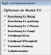
The sound level calculation for compressible and incompressible media is based on VDMA Guideline
24 422, January 1989 edition.
Unsteady flow - e.g. when opening a valve or changing the upstream pressure- is calculated according to "Mechanics of Fluids", Potter/Wiggert, Prentice Hall 1997.
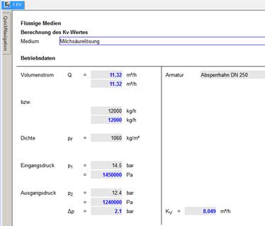
For incompressible media, the calculation is performed in the mask shown below. After entering the required values, the result is automatically calculated and entered.
In the following section you will find more information about calculation with compressible media, steam and two-phase flow.
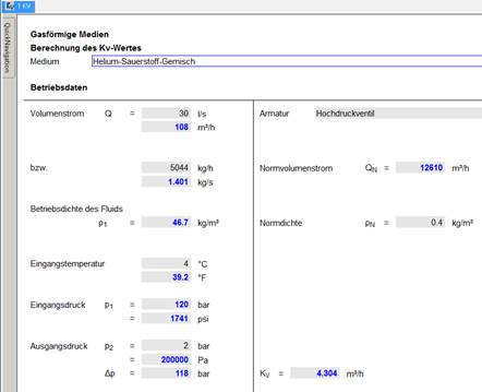
After starting the module, select the option "Kv gaseous". Enter the known data in the input mask.
In the following example, the values shown in black were entered by the user, the values shown in blue were calculated by the program. However, it does not matter which values are entered.
As soon as sufficient values have been entered, the program automatically calculates the missing values according to the stored formulas.
|
The
calculation for saturated steam or wet steam and superheated steam takes
place after clicking on
|
|
|
|
|
|
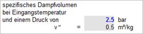
When calculating Kv for steam, it is necessary to specify the specific volume of steam at the calculation pressure:
|
|
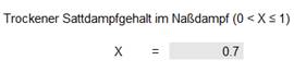
To calculate the Kv value, the Kv value for the liquid and gaseous components is first determined separately. To obtain the total value, these two values are added and multiplied by the correction factor to be entered for two-phase flow.
The correction factor is in the range 1..2.
Correction factors for fittings connected to the valve, etc. (factor for pipe geometry), for turbulence (Reynolds number factor) and pressure recovery are not considered in this module. This means that turbulent flow is generally assumed - as is usually the case in control valves. Connected components cannot be taken into account.
The calculation masks for sound level calculation have been adapted to the templates in VDMA Guideline 24422. Thus, the calculation is analogous, the documentation - i.e. the printout of the masks corresponds in structure to the calculation sheets.
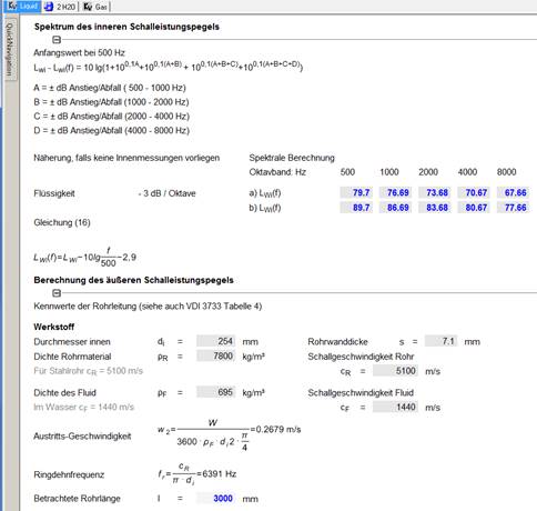
Detail of the mask
The calculation of the closing behavior of a valve can be found under Closing behavior of a valve .
The calculation of unsteady flows is performed in this module exclusively for incompressible media.
The steady-state initial condition must be specified, i.e.
· the hibernation state
In this case, initial velocity or initial flow rate are zero;
or
· an initial flow value
Example:
Starting from a certain flow rate, the upstream pressure is increased. After which time
· does the stationary state re-establish itself?
· is a certain flow rate achieved?
· 95 percent of the final speed has been reached?
Further studies, e.g. on the dependence of a parameter on two other parameters, can be carried out using the parameter study in the ATLAS menu item.
A liquid with a given density is conveyed in a pipeline with an inner diameter of 500 mm and 60 m length. The relative roughness of the pipeline is 0.00107, and the initial steady-state flow rate is 10 m³/h.
A fitting with a value.fitting = 0.8 is installed in the pipeline.
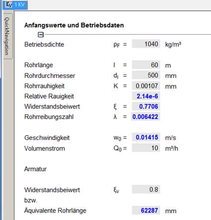
For the transient calculation, the following question is asked:
How do the flow conditions change when the upstream pressure, i.e. the effective pressure difference, is increased by 0.5 bar?
To do this, enter the corresponding value in the lower area of the mask (shown in black letters):
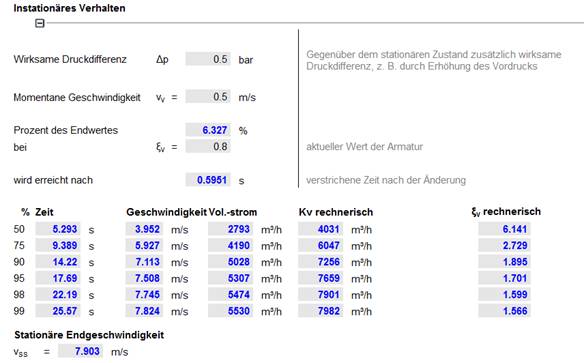
The values shown in blue were calculated by the program.
Note:
The time for reaching 50 percent of the final velocity is given as 0s. The initial velocity in the stationary initial state was already higher than the corresponding velocity. Only at the initial velocity (or initial flow) zero, all values always become greater than zero.
With the same input values, only the achieved steady-state final velocity was specified in the following example. Accordingly, the additional pressure difference and the values in the table are calculated automatically.
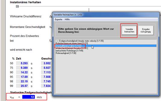
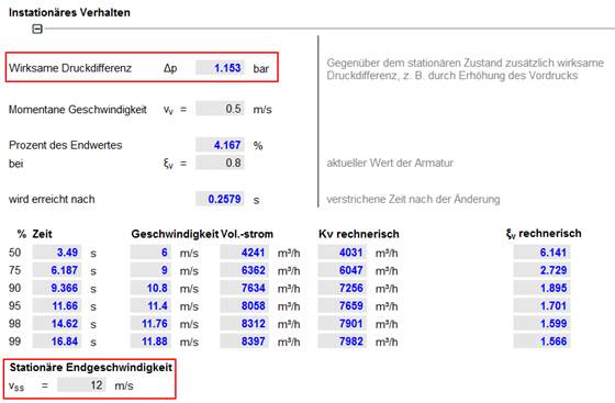
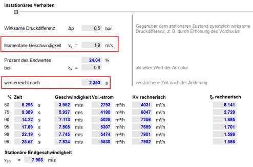
In the area above the table, any intermediate steps can be calculated. For example, specify a pressure increase of 0.5 bar and calculate the values at a velocity of 1.9 m/s achieved:
In the example - entered in blue - this speed was reached after approx. 2.4 seconds. The flow rate is 24 percent of the final value.
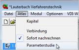
A wide range of calculation options is offered by the Parameter Study option in the ATLAS menu
|
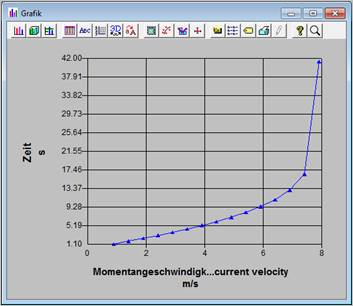
Here you can perform various kinds of two- and three-dimensional dependency studies and view the results as a graph, save them as an EXCEL table ...
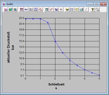
Example of a graph (parameter study):
|
|
|
|
For more information in the general ATLAS manual.
|
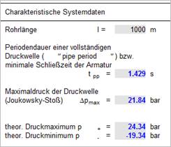
Here you calculate the maximum pressure surge when closing a valve and the reduced pressure surge according to the specified closing time. In addition, the pressure losses of the pipeline and the valve in steady state are calculated. If the vapor pressure of the fluid is known, it can be assessed whether cavitation occurs when the valve closes.
This calculation is performed exclusively for incompressible media. The sound velocity of the fluid must be specified.
For a given valve closing time, the height of the corresponding pressure wave is calculated:
|
|
|
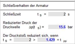
Among other things, this module also calculates the pressure loss values of a steady flow:
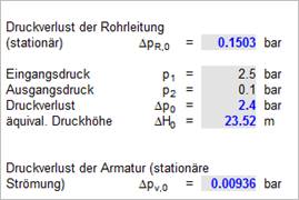
If the vapor pressure of the fluid is known, the calculation of the minimum static pressure can be used to determine whether cavitation will occur as a result of closing the valve.
By means of parameter studies, the occurring pressure surge can be calculated as a function of the valve closing time as one of many possibilities.