Structure and operation
The program consists of units (modules) of the ATLAS program system, which are linked with each other by the input and output variables. Every module represents an independent program provided with an input/output surface.
From the main operating surface (AC) or from any module it is possible to get to the operating surfaces of the various modules by the pull-down menu ‘ATLAS’ – ‘Chapter’ – (Name of the module).
The following modules are available for use in AC:
|
Module |
Standard |
Extra Charge |
|
|
Bare tubes inside/outside |
|
X |
|
|
Circular finned tubes (Tube outside) |
|
X |
|
|
Spiral fins with ripples (Tube outside) |
|
X |
|
|
Rectangular finned tubes / fin plate |
|
X |
|
|
Tube register |
|
X |
|
|
Rectangular multi-pass shell |
|
X |
|
|
Round tubes / Oval tubes |
L1.4 |
X |
|
|
U-tube / Straight tube |
|
X |
|
|
Steady-state temperature distribution |
ZELL |
X |
|
|
Internal longitudinal or spiral fins |
INLR |
|
X |
|
Twisted tape inserts |
TWIS |
|
X |
|
Round multi-pass shell |
L1.5 |
|
X |
|
Corrugated tubes |
DRLL |
|
X |
|
Natural convection |
ACK |
|
X |
|
Pool heat exchanger (free convection / no circulation) |
F2.1 |
|
X |
|
Construction types |
Module |
Standard |
Extra Charge |
|
Recirculation of hot air |
PLRE |
|
X |
|
Power consumption of fan |
VENT |
|
X |
|
Unsteady-state temperature distribution (transient) |
ZELL Trans |
|
X |
|
Physical properties |
|||
|
Ammonia (evaporation / condensation) |
NH3 |
X |
|
|
® Antifrogens N, L, KF and SOL |
GLYC |
X |
|
|
Free input of properties |
S-DAT |
X |
|
|
Hydrogen - Nitrogen - Mixture (Cooling gas) |
H2N2 |
X |
|
|
Air (dry / humid) |
LUFT |
X |
|
|
12 typical machine oils |
OEL |
X |
|
|
Flue gas / Process gas |
RGAS |
X |
|
|
Saturated steam |
H2O |
X |
|
|
100 thermal oils |
T-OIL |
X |
|
|
Water and steam |
H2O |
X |
|
|
Refrigerants |
FRIG |
X |
|
|
Carbon dioxide |
CO2 |
|
X |
|
Natural Gas L, H and any composition |
EGAS |
|
X |
|
Nitrogen |
N2 |
|
X |
|
Nitrogen-Hydrogen-Carbon monoxide-Mixtures |
Gasmix |
|
X |
|
Helium |
He |
|
X |
|
Properties of pure substances and mixtures |
PROP* |
|
X |
|
User-supplied properties tables |
S-TAB |
|
X |
|
Miscellaneous |
|||
|
Tube sheet as DXF |
|
X |
|
|
Customer documentation (abridged) |
KUDO |
X |
|
|
* requires LV program PROPER ® Registered trademark of Clariant GmbH |
|
|
|
There is no difference between a separate data input process and the calculation process. The program system ATLAS is a simultaneous dialogue/calculation system. Every value entered immediately leads to a processing step as long as the system is specified and the solution is found. The user himself can decide which value is a set value and which value is a result.
The basic functions of this module and how to work with it are described in the manual for the ATLAS program system.
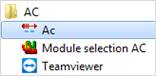
After starting the program by ‘Start / programs/ AC / AC’ the mask for selection of media and for further specifications appears
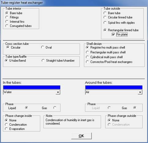
Selection menu (example)
In the top section the geometrical data of the tube is specified.
In the center section the geometry of the heat exchanger is specified.
The options ‘Fittings’, ‘Internal fins’ and ‘Corrugated tubes’ as well as ‘Multi-pass shells’ and ‘Pool heat exchangers’ are only active if the respective additional modules are installed and unlocked.
In the bottom section the mass flows in and around the tubes are specified. The user can enter the phase (gas, liquid) of the media as well as a phase change (condensation, evaporation). If humidity condenses from an inert gas (e.g. wet air, flue gas) select ‘none’ for phase change. Condensation of the humidity is considered anyway.
‘Water’ is set as default medium in the tubes and ‘air’ as default medium around the tubes. To select another medium, open the medium selection window. After selecting the media, the properties are calculated automatically by the corresponding modules (e.g. air, water). Please note that some of the media mentioned in the example are not included in the basic package of AC.
If ‘Free input’ has been selected as medium, the properties have to be entered manually. After confirmation of your selection by ‘OK’, the main operating surface of the module AC appears. To get to the operating surfaces of the various modules use the menu item ‘Chapter’ of the ‘Atlas’ menu, which is described in the manual for the ATLAS program system.
The operating surface of the AC module provides almost all the input options required for the calculation of a heat exchanger. These input values are displayed in the corresponding modules as well. The user controls the run of the calculation from the AC operating surface. From here it is possible to switch to all other modules.
|
Different from all other Atlas modules, AC provides a menu named ‘Special’ which can be found in the menu bar of the input mask. The menu item ’Tube sheet’ is only available if there are enough geometrical values in the input and output mask of AC. With the menu item ’Natural convection’ (*) an air cooler designed earlier can be converted from forced convection to natural convection by mouse-click. |
|
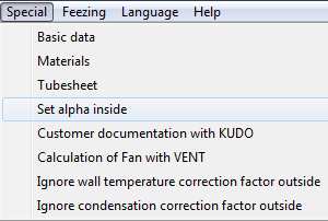
The menu item ’Calculation of Fan with VENT’ (*) transfers the calculation of the fan performance to the VENT module, where you can for example enter the fan efficiency. By default the fan performance calculation is performed by the AC module.
*not included in the standard package
|
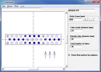
After input of all geometrical data of the bundle the tube sheet of the bundle can be opened by ‘Special’ / ‘Tube Sheet’ After loading an SPI file (SPI means tube sheet) the editable text fields in the window ‘Tube sheet‘ display all information about type and dimensions of the tube sheet saved in this SPI file. Above the graphic there is a text field where the name or description of the tube area can be entered. In the text field to the right of it the name of the SPI file is displayed. |
|
||
|
|
|
||
|
In the menu bar of the window ’Tube sheet’ the ’File’, ’Zoom’ and ’Print’ menus can be found. With the ’File’ menu you can load SPI files, save the tube sheet as SPI file or leave the window ‘Tube sheet‘ with ‘End’. With the ’Zoom’ menu the outside frame of the graphics window can be reduced or enlarged. With the ’Print’ menu you can print your tube sheet on your printer save it as DXF file for further processing with a CAD program (e.g. AutoCad). After selecting ‘Printer’ the mask ‘Layout’ appears.
|
|
||
|
|
|
||
|
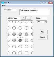
In the ’Print’ menu of the ’Layout’ you can specify to have the tube sheet printed on one, two or four pages (DIN A4). With the buttons + and - you can switch between these pages. The current page is always displayed. With the selection menu ’Scale’ you can adapt the tube sheet to the size of the page(s) by clicking on another scale. The change of the scale immediately modifies the displayed page.
|
Export tube sheet
|
||
|
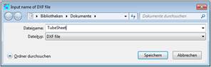
In the field ’comment’ a text can be entered. This text, the file name (SPI), the scale and the number of pages appear on the printout. After printing the tube sheet, the mask ’Layout’ is closed. With the button ’Cancel’ you can abort the processing and leave the mask without printing. After selecting the menu ’Print’ + ‘DXF_file’ menu a window appears where you have to enter the name of the DXF file. |
|||
In tube registers, the hat transfer coefficient outside the tubes is corrected with a factor, calculated by the ratio of mean outside temperature and wall temperature. If you ignore this correction, the factor is set to 1.
By shell side condensation of humidity, the heat transfer coefficient improves. This improvement is considered by a factor, calculated by an arithmetic approach developed by LV. It is also considered that the condensation takes place at the subcooled wall and that it is possible that the medium is not saturated. If you ignore this correction, the factor is set to 1.
You can perform a user-defined correction by changing the value of the ’engineering factor: Heat Transfer’.
As a matter of principle it is possible to enter data in any order. The target of the calculation is always reached, even in a roundabout way.
|
We recommend selecting the tube and bundle data first and then determining the heat balance. |
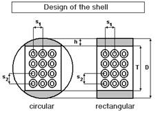
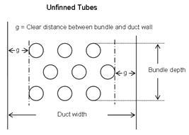
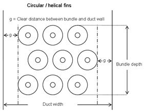
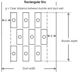
The cross flow bundle consists of tube rows with an equal number of tubes. The arrangement of the tubes (tube sheet) is determined by the pitch in longitudinal and crosswise direction and by the position (aligned/staggered or partly staggered). All these options can be selected.
For finned tubes the dimensions of the fins are required. The tube diameters, the length and the number of passes conclude the definition of the geometry.
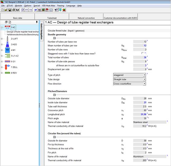
By selecting ‘Special‘ / ‘Tube sheet’, the specified geometry of the bundle can be viewed true to scale.
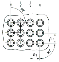
The crosswise pitch of the tubes is the center-to-center distance of the tubes in a row.
For bare tubes a good reference value is 1.2 to 1.3 times the tube outside diameter.
The longitudinal pitch of the tubes is the center-to-center distance from one tube row to the next tube row.
Crosswise pitch and longitudinal pitch are related to each other by the pitch angle (0-90°).
Staggered longitudinal pitch:
If the tubes of a row are not situated exactly in the center of the gaps in the next row.
|
Aligned |
Staggered |
|
|
|
|
Staggered |
Staggered |
|
|
|
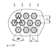
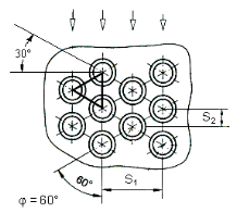
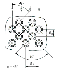
Partly staggered
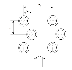
This is the number of tubes in the first row from the outer medium‘s perspective
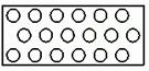
With a staggered tube arrangement, either each row has the same number of tubes, which results in an asymmetrical tube sheet,
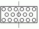
or every staggered row has one tube less than the row before, which leads to a symmetrical tube sheet.
|
How many times does the medium inside the tubes pass the bundle? |
Example:
The medium enters the bundle, passes it once, is turned round at the end, flows
back, is turned round again and leaves the bundle after a last pass. That makes
three tube side passes.
The number of tube side passes has an influence on the velocity of the medium. The faster it flows the higher the pressure loss. But on the other hand also the heat transfer inside the tube gets better.
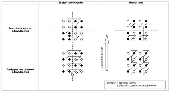
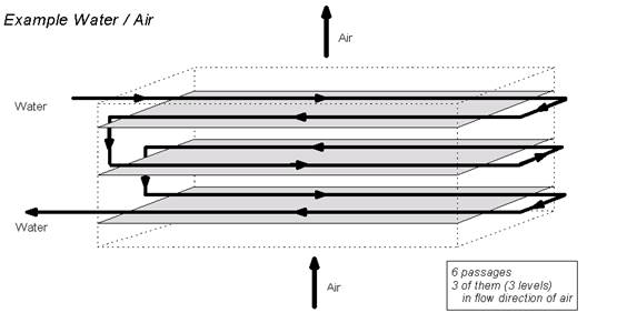
The number of steps in which the tube side medium is led against the direction of the flow of the outside medium.
The number of passes in direction of flow around the tubes determines, how much the countercurrent-effect is influencing the thermal behavior of the exchanger. Remember that air coolers (or any exchanger similar to this) are usually built as countercurrent-cross-exchanger. The more passes in direction of outside flow you have, the more dominates the countercurrent behavior (which is thermodynamically favorable).
If there are more tube rows then passes, you usually lead the inside medium with all passes towards the outside flow.
Are there, on the other hand, less tube rows then passes, you have to lead some passes crosswise to outer flow direction. That means, for example in a horizontal air cooler, that you have to braze some U-fittings horizontally.
For mass flows which are not subject to a change of phase the inlet pressure, the inlet temperature and the outlet temperature are required for automatic calculation of the properties.
For condensation or evaporation processes of pure substances either the inlet pressure or the inlet temperature may be predefined. Using a steam pressure curve, the program calculates the missing state variable and the properties automatically.
If the desired mass flow is not
selectable in the ‘Tube register heat exchanger’ selection menu
(Fig. 2.2) the medium has to be defined as ‘Free input’ and the
properties have to be entered manually. Please make sure that the properties
are defined for the mean temperatures.
Please note the following procedure:
Enter the mean temperature and the pressure of the ‘Free input’ in the input/output mask of AC. The program automatically creates a chapter SDAT and switches to it.
Enter the properties for ‘state 1’ there, in the following order
1. Density
2. Specific heat capacity
3. Dynamic viscosity
4. Thermal conductivity
After input of the heat conductivity the program switches to the module AC automatically (while applying the entered properties).
Enter the relative humidity or water content for air. To enter a relative humidity does only make sense for temperatures below the boiling point of water. For higher temperatures the air might comprise an arbitrary amount of steam. Then you need to enter the water content (load) only.
For flue gas the water content is determined automatically. Condensation due to subcooling below the dew point is considered.
The heat balance determines the nominal performance of the heat exchanger. Temperatures, pressures and flows are entered in the AC program mask in any order.
To determine the balance it is necessary to give five values of the four temperatures (two inlet and two outlet temperatures) and two steam flows. The sixth variable is determined by the program and can't be selected freely.
In case of an unknown temperature a fictive value has to be entered so that the program can switch to the relevant material chapter.
If all four temperatures are given and the mass flow of one side (e.g. in the tubes) is known, the mass flow of the other side (e.g. around the tubes) is calculated by the program to close the heat balance.
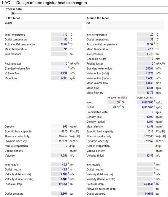
AC input mask - properties and heat balance
As soon as all data are available to determine the heat balance, the program calculates a ‘thermal performance (actual)‘ on this basis.
The comparison with the ‘required thermal performance’ from the heat balance shows if the predefined bundle meets the requirements or not.
Performance factor (= ’Thermal performance (actual)’ / ’Thermal performance (required)’)
If the performance factor is less than 1 the heat exchanger is undersized, if it is greater than 1 it is oversized.
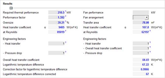
AC input mask, Evaluation
To adjust the exchanger to the required thermal performance, you have the following possibilities:
1. You may modify the geometry or the process conditions to adapt the performance. This depends on the specific type of problem and on the boundary conditions.
2. Another possibility is provided by the parameter study or the Scenario Manager. The user can plot the performance factor as a function of any variable (e.g. tube length) and size the exchanger or evaluate its performance under modified process conditions.
For evaluating the design of a heat exchanger, usually a value is used which shows the ratio of actual thermal performance and required thermal performance. These are an area reserve, an oversize or a performance factor. The AC program states the last two.
How is the oversize calculated?
First the required thermal performance Qsoll is calculated. In case of single-phase flow it results from the mass flow, the specific heat capacity and the temperatures of one of the flows.
In comparison to this a theoretical thermal performance is calculated, which results from the required conditions.
With k: Heat transfer coefficient
A: Outer exchanger area
FN: Correction factor due to flow pattern (Deviation from pure countercurrent flow)
ΔTlog: Logarithmic mean temperature difference
These two performances are used to form the two evaluation values:
Performance factor 
Oversize  (stated in percent)
The equations show that both values are only different presenting variants of the same fact. Therefore all following statements are valid as well for the performance factor as for the oversize.
How to interpret the evaluation values?
First the simple case: An Oversize of 0% (Performance factor of 1.0) means, that the exchanger is designed to the point. It has exactly the demanded thermal performance, provided that all assumptions for the design were correct.
An Oversize of 10% means that with a deviation of the influence values of 10% downward, the exchanger has exactly the demanded thermal performance.
For example, due to the inaccuracy of the mathematical approaches the k value might be smaller than assumed, there is a heat loss or the fin area is smaller than calculated due to manufacturing tolerances.
Then the oversize brings a certain safety that the exchanger fulfills his task anyhow.
An Oversize of 10% does not mean that the exchanger transfers 10% more heat if all assumptions are correct. In this case there is a deviation from the specified condition and influence values of the heat transfer do change. Especially the driving temperature gradient may become smaller with partially great effects.
This fact is considered when calculating the actual outlet temperatures according to the cell method in the ZELL module.
At the same time as the thermal calculation the program determines the pressure loss in and around the tubes as well as both outlet pressures.
The user can compare the calculated
pressure losses to the allowed pressure losses (given values).
If necessary he can modify the input values (e.g. geometry values) to satisfy the boundary conditions or modify an input value
by entering the desired pressure loss.
With the parameter study (see ATLAS manual) the calculated pressure loss can be displayed as a function of the input values (e.g. variable process conditions: temperatures, throughputs).
The outside medium flows through the bundle several times.
In rectangular shells it is turned around in a chamber, which may be very individual in geometry. Therefore the calculation of the pressure loss due to the deflection is only possible by using a pressure loss factor (friction factor). Normally you can assume a value of 0.5 to 5.0. The given value has only influence on the calculation of the shell side pressure drop.
(For examples see also: Renknagel, Sprenger, Schrameck, ‘Taschenbuch f. Heizung und Klimatechnik)
In most cases you calculate the exchanger with an overdesign. That means it transfers more heat than demanded. The outlet temperatures in reality are thus different from the temperatures assumed in design. The actual outlet temperature is the temperature in the real process.
Particularly in designing multi-stage exchangers (e.g. two circuit coolers) it may be important to know the actual outlet temperatures of the primary stage.
The engineering factors allow you to correct the calculated values for the pressure drop and heat transfer, based on your own engineering experience. If you use for example a special type of fin, the actual heat transfer might be better than the one calculated according the general calculation approaches. You may then enter an engineering factor of 1.1 for example ( = the heat transfer is enhanced by 10% compared to standard fins).