Operation of the program

The application is started by executing the Good Vibrations.exe file in the Explorer or by selecting GOOD VIBRATION from the Start and Programs menu with the mouse pointer.

After starting the program, the graphical user interface is displayed (Fig. 1). In a separate window, the input of project-related data is possible. The input mask of GOOD VIBRATIONS consists of five tabs, in which the input data are to be entered one after the other. Through the tabs, the input data are thematically separated according to

·       Geometric sizes

·       Material and substance values

·       Pipe mirror

·       Intermediate supports

·       Calculation specifications

·       Optional specifications

The designation of the quantities to be entered is done according to the nomenclature of the section Oc in the
VDI Heat Atlas [1].

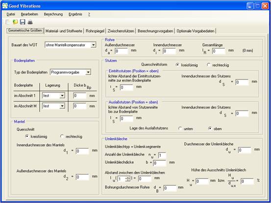
Figure 1: Basic mask  

In the Geometric sizes tab, shown in Fig. 2, all values for the geometry of the shell, the pipes, the nozzle and the baffles are entered and information is given on the design of the cross-flow device. Circular or rectangular cross-sectional shapes are possible for the shell and nozzle. In the case of rectangular cross-sectional shapes, the dimensions of the shell or nozzle in the x and y directions or in the y and z directions must be specified.

By specifying the edge supports, the number of baffles nU, the spacing of the baffles lU and the segment cutout height _{HU, the} support conditions of the individual tubes and the flow sections are determined. The total length of the pipes must correspond to the sum of the distances of the baffles and the bottom plate thicknesses.

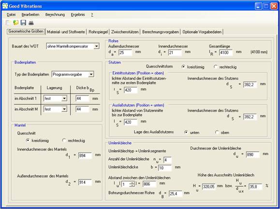
Figure 2: Geometric quantities

The position of the first segment cutout is at the bottom. The cutouts in the other baffles are alternately at the top and bottom.

Top indicates the cross-sectional half of the heat exchanger where the inlet nozzle is located (Fig. 3).

§   The inlet nozzle is always in section 1, the outlet nozzle in section M.

§   The segment cutout height is defined between the baffle edge and the inside diameter of the shell.

§   The distance of the baffles is specified up to the center of the respective baffles. For the first and last baffle, the distance from the center of the baffle to the base plate surface must be specified. Furthermore, the diameter of the baffle, the baffle thickness and the bore diameter in the baffle for the pipes must be specified.

Warning:

Enter number of baffles first. If _nu is changed later, all values that depend on the number of the flow section are reset.

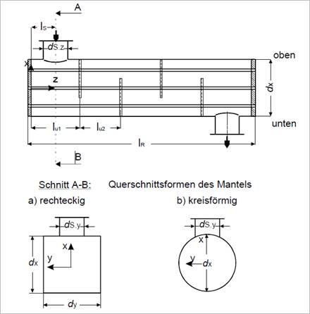
Fig. 3: Sketch of the geometric dimensions and cross-sectional shapes of the heat exchanger

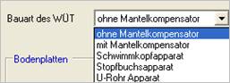
The calculation of structural data for U-pipes is provided, but in the current version it is possible alternatively only with structural data for the straight pipe sections or by specifying optional data.

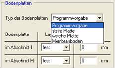
Depending on the type of base plates (Fig. 5), the program determines the plate stiffness, separately for inner and outer tubes, approximately for the calculation of the axial tube force [1,Tab.6]. Deviating from this, the stiffness factors XI for inner tubes and XA for outer tubes can optionally be specified (see tab optional specifications, Fig. 13).

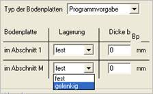
The bearing conditions of the tubes in the base plates are decisive for their natural frequency and the vibration mode. The possible choices of tube support in the base plates are shown in Fig. 6. For the baffles, an ideal articulated bearing is assumed, i.e. approx. 8 - 20 mmwide, well rounded and with the smallest possible bore clearance.

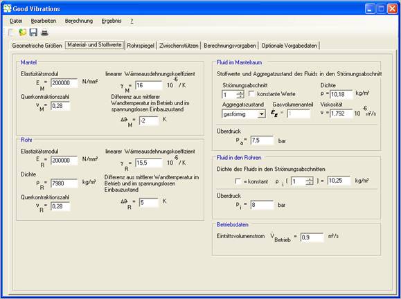
Figure 7: Material and substance values tab

The input mask for the material and substance data of the jacket, the pipes and the flow media is provided with the Material and substance values tab (Fig. 7). The density ρ of the fluids in the pipes and in the shell space as well as the state of aggregation, the viscositynand, in the case of two-phase fluids, the gas volume flow rate εg in the shell space (Fig. 8) can be specified separately for all flow sections.

In case of constant material data in all sections of the jacket space, the input of a constant value for the respective quantity by activating checkbox constant is sufficient. If the aggregate state two-phase is selected, the program currently calculates with the equations for liquid flows.

More precise critical velocities can be determined from the VDI heat atlas and optionally specified.

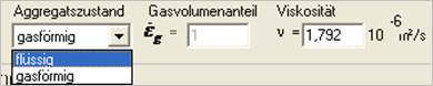
Figure 8: State of aggregation list box

The automatically generated pipe surface is displayed in the Pipe surface tab (Figs. 9 and 10). For this purpose, the pipe pitch angle, the pipe pitch ratio or the pipe pitch and the desired enveloping circle diameter must be specified.

Pipe rows can be removed as follows:

§   from above in the upper half of the mirror

§   from below in the lower half of the mirror

§   in the center of the bundle.

The symmetrical arrangement of the tube rows with respect to the center of the mirror can be specified: 

Checkbox 'Exists a center pipe' (Fig. 9).When loading input files, the pipe mirror is calculated and drawn automatically.

The tube rows to be calculated with regard to the vibration hazard are highlighted in color. By default, all pipe rows of the heat exchanger are calculated in the program. Individual tube rows can be calculated by unchecking the Calculate all tube rows checkbox and selecting the tube row to be checked in the list box. The number of tube rows, the total number of tubes and possibly (in case of a tube row to be calculated) the number of tube rows in the respective window and the vertical distance of the tube row to be calculated to the bundle center are displayed.

In the event that the automated pipe level does not match reality, the total number of pipes can be corrected. The corrected value is only taken into account in the calculation of the axial forces. The pipe surface drawing is not changed by this in the present version.

Since the vibration hazard is always based on pipe rows completely filled up to the shell, i.e. on the maximum possible load of the bundle, an exact agreement between the calculated and the real pipe level is not decisive as long as the agreement of the chord lengths of the considered pipe rows is given.

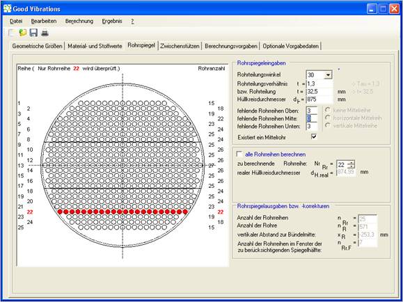
Figure 9: Tab pipe mirror, cylindrical shell

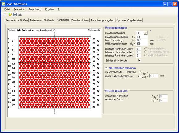
Figure 10: Tab pipe mirror, rectangular shell

In Figure 11, 3 pipe row blocks have been defined.

The 1st block RBB(1) includes a partial support grid for the 1st to 5th row of pipes, e.g. for the rows of pipes under the inlet spigot.

The 2nd block RBB(2) is a support grid that encloses all pipe rows of the bundle from the 1st to the 31st pipe row.

The 3rd block RBB(3) includes a partial support grid for the 27th to 31st row of pipes, e.g. for the rows of pipes under the outlet spigot.

For each tube row block, the number of intermediate supports and the length of the support section lu can be specified in each flow section. The length of the support section always refers to the previous baffle or tube sheet or to the previous intermediate support. The distance between the last intermediate support and the next baffle cannot be specified.

In order to be able to enter the length of the support sections, the Constant spacing checkbox must be deactivated.

In the present example, the pipe row block RBB(1) (partial support grid) was placed only under the inlet nozzle, i.e. the number of intermediate supports in the 1st flow section is 1, inall other flow sections the number of intermediate supports is 0.

The pipe row block RBB(2) was placed between the baffles, i.e. in the 1st and 5th flow section the number of intermediate supports is 0 and in the flow sections 2 ,3 and 4 each 1.

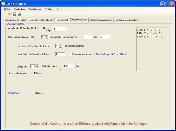
Figure 11 - Intermediate supports tab

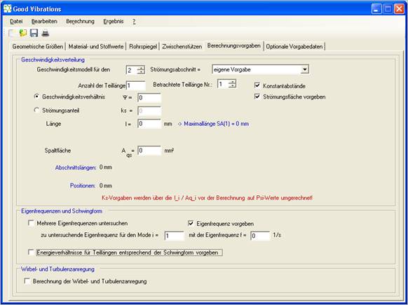
Figure 12: Calculation specifications tab

In the Calculation Defaults tab (Fig. 12), the check of vibration excitation by vortex and turbulence excitation can be switched on or off. Furthermore, the number of natural frequencies to be examined can be set. If several natural frequencies are to be considered, the highest mode to be considered must be specified (default setting i=1-6). If only one natural frequency is to be analyzed, mode i of the natural frequency must be entered. For this mode an own specification for the natural frequency can be made, the vibration mode and the energy ratios are calculated by the program. However, you should make sure that the preset natural frequency and the calculated oscillation mode are compatible. In the standard default setting, the vibration excitation due to vortex and turbulence excitation is also determined; the first six natural frequencies are used for the determination of the vibration hazard.

The velocity distribution can be defined by specifying the relative velocity ratio yor by specifying the flow fraction kS for each partial length. If the flow proportion kS is specified for each partial length r, the following must apply:

S kS,r = 1

The velocity distribution in the pipe gaps along the pipe axis can be selected for each flow section. With the default setting (program default), the program automatically determines the distribution of the equivalent velocity for a cross-flow apparatus taking into account the models according to Mohr [3,4]. This always takes effect if all pipe rows in the heat exchanger are examined.

Deviating from this, three different velocity models can be selected for a given pipe series:

homogeneous distribution, jet inflow [1] for the first and possibly the second row of pipes and the nozzle model according to Mohr [3] for the second or third row of pipes for the nozzle inlet and possibly the nozzle outlet area (Fig. 12a).

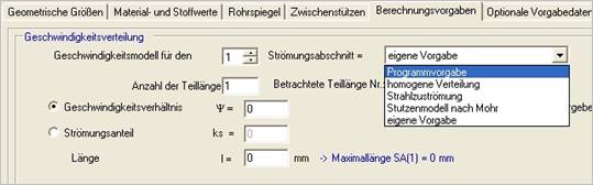
    Fig. 12a: Calculation specifications / velocity models tab

Furthermore, for a given pipe series, the velocity distribution can be freely specified in the form of a staircase function in which the velocities in each partial section are constant; it should be noted that the sum of the partial lengths is equal to the width of the flow section under consideration.

Fig. 13 shows the information required for your own specification of the velocity distribution for a given pipe series, the number and length of the flow areas of equal velocities and their associated value of the distribution function. Furthermore, the size of the flow area must be specified.

If no value is inserted for the flow areas, then automatically for the flow sections the gap cross section areas are calculated from the length of the section and from the chord length of the considered pipe row i.e. normally too large. The course of the distribution function in a flow section is specified by the input of relative values, i.e. only the relations of the values for the individual flow section are considered, the true values are calculated via the continuity equation for the volume flow in the program.

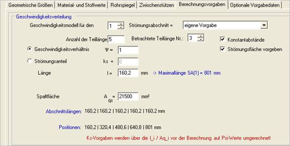
Figure 13: Speed distribution list box

If a separate distribution has been specified for all flow sections, it is still possible to perform the calculation without the automatic determination of the natural frequency and the vibration mode.

For this purpose, the check box 'Specify energy ratios for partial lengths according to oscillation shape' must be activated (Fig. 13a).

In this case the mode i, the natural frequency as well as for each partial section of the velocity distribution the partial energy ratios have to be preset. The input is the same as for the velocity specification, but the natural frequency must be entered in advance and a separate specification of the velocity distribution must be selected for each flow section.

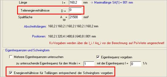
Fig. 13a: Partial energy ratios

In the optional default data tab, the default settings in the program can be changed (Fig. 14). This may be necessary if deviating designs (e.g. longitudinal flows) or changes in condition are to be taken into account.

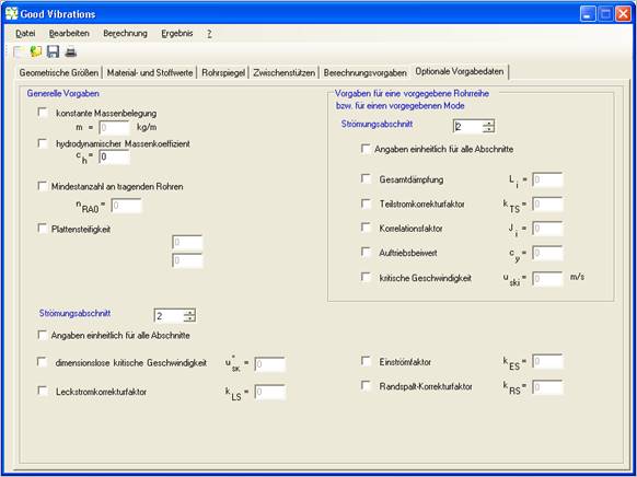
Figure 14: Optional default data tab

A distinction is made between default data that is valid for all pipe series or only for a specified pipe series / for a specified mode.

For all pipe series and independent of the oscillation mode can be specified:

·       Total mass occupancy m or the hydrodynamic mass coefficient _ch for variable mass occupancies.

·       Minimum number of pipes n_RAO on axial load bearing pipes:

Standard values for cylindrical shells see [1], exact values by counting the edge tubes in the tube sheet, absolutely necessary for rectangular shells

·       Plate stiffness X_I and X_A

For default values see [1, Tab.6,]

and for each flow section:

·       Leakage current factor kLS records the cross-current component (also > 1 possible):

To take into account changing mass flows, e.g. during condensation or evaporation or in longitudinal flows. The gap losses of the baffles are normally calculated automatically, but are overwritten by a default!

·       dimensionless critical velocity:

The critical velocities are calculated automatically in the program depending on the arrangement, the pipe row and the mode i, taking into account the inflow conditions and the edge gaps. However, the oblique flow must be taken into account in the default value according to [1, Tab.11].

Only for a given pipe series it is possible to specify the following in deviation from the standard calculation in the program:

·       Inflow factor k_ES:

e.g. when specifying an own inflow velocity distribution; default values [1, Tab.11],

·       Edge gap correction factor k_RS,

which takes into account the influence of the edge gap on the shell during accelerated flow,

and for each flow section:

·       Total damping λi :

valid for the given mode i resp. constant for all modes

·       Partial current factor kTS ( < 1 ):

is automatically calculated for the inflow volume flow of the window pipes,

·       Correlation factor J_i:

for turbulence excitation at a given mode; standard values [see 1.5],

·       Coefficients of buoyancy cy:

for vortex excitation, standard values for bundles and single tubes (τ > 3.5) see [1, Oc17],

·       critical speed in the real bundle u_ski:

only for the given mode i, is accepted without further corrections

If no values are entered in the corresponding fields, the program determines these values.

After entering all data, the calculation can now be started. To do this, select the Start menu command from the Calculation menu (Fig. 15) to run the calculation with the mouse. During the calculation, the status of the calculation is displayed in a new window.

After the calculation is finished, a result file with the extension *.gva is created.

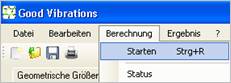
Figure 15: Calculation menu

After the calculation is finished, the results can be displayed on the screen. To do this, select the Display field in the Results menu (Fig. 16) with the mouse pointer. The results are read from the result file *.gva. A new window with the results is opened, the first page contains a summary.

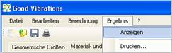
Figure 16: Result menu

The Print command in the Result menu (Fig. 16) prints the result file on the printer. The appendix contains examples. For editing and saving the printout, programs such as Adobe Acrobat or MSOD Image Writer are recommended, which are called via the Print command.

On the first printout page, Fig. 1 shows the pipe level and, highlighted in color, the checked pipe row(s) or all calculated pipe rows. The highest calculated degree of hazard for fluid-elastic instability and the maximum amplitudes for stochastic and periodic excitations are listed and evaluated together with the corresponding pipe rows, natural frequencies and critical volume flows and velocities. This is followed by the input data and the geometry data, material and substance values, structural and operating data calculated from them.

In the first part, the detailed results regarding the vibration hazard due to fluid elastic instability are described. First of all, the bearing conditions as well as the structural, material and critical data for the investigated or the endangered pipe series are listed. In Table 1 of the printout, the intermediate results of the calculation are output section by section for the given or the critical natural frequency. The sum of column 8 intable 1 determines the degree of endangerment, so that from the sizes of the proportions in column 8 the dominating sections can be seen, where constructive measures for improvement would have to be carried out under certain circumstances. The sum of column 8 results in the maximum critical velocity and the critical inlet volume flow of the heat exchanger for the examined tube series. Furthermore, the degree of danger - the stability ratio K* of the bundle - is output, which results from the ratio of operating volume flow to critical volume flow.

The program-internally calculated or preset velocity distribution is shown together with the critical oscillation mode in Figure 2 of the printout. The user can check the realism of the specifications and, if necessary, change them in a new calculation. The result is then evaluated and the hazard levels for the next two endangered pipe rows or specific modes are listed. Further notes and warnings, e.g. regarding the range of validity of the equations used, follow.

In the second part, the results are described with respect to the stochastic and periodic excitations, if desired. The results are shown for the given pipe series or for the pipe series most exposed to turbulence and vortex excitation, which may differ from the most exposed pipe series due to fluid-elastic instability.

First, the data dependent on the storage conditions: Natural frequencies for the considered modes (see also Table 3 in the printout), the Strouhal numbers and the critical resonance velocities for which excitation could be considered. The resonance distance as well as the Reynolds number limits and the validity ranges for the Strouhal numbers are taken into account (e.g. the validity of Sr_w,2 only in the entrance range for m=1).

Table 2 in the printout contains the velocity distribution and the operating velocity for the considered pipe series as well as, as intermediate results, the weighted vortex excitations in the subsections for the six modes with the highest hazard levels. The square root of the sums of columns 5 to 10, possibly taking into account the correlation factor J_w,i,m [1] result in the amplitude maximum values A_w,i / d_a in table 3. Therefore, the sizes of the proportions in columns 5-10 of table 2 indicate in which subsections the largest periodic excitations occur.

Table 3 summarizes the results for vortex and turbulence excitation. It contains representations of the investigated vibration modes and the associated maximum amplitude values for vortex as well as for turbulence excitation and, as degree of hazard, the maximum values from the summed modes, which are also shown.

The results are evaluated and the hazard levels for the next two rows of pipes at risk are listed under Notes.

The toolbar contains the buttons for  access to the commands Create New File, Open File, and Save File.

In the File menu (Fig. 17) of the menu bar the menu items for file management are arranged and allow to create, open and save a file with the input data. With the references to the last opened files, they can be opened immediately. The application is closed with the Exit command.

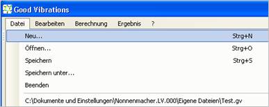
Figure 17: File menu

The Save command saves the input data to a file with the extension *.gv. These files can be accessed again later with the Open command. All entered data and information are saved. The New command creates a new project and resets all values to the default settings.