Operation
The LV-PIPE II calculation system consists of several components. The user interface is an Excel add-in. The calculation modules, the CAD module and some auxiliary modules are ActiveX components. The latter work essentially in the background.
>> Before the system can be used, it must be installed on the corresponding computer.
|
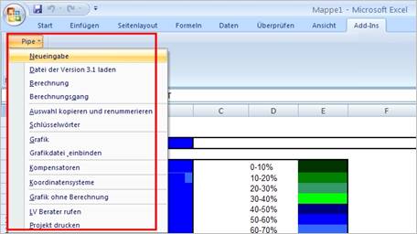
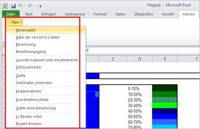
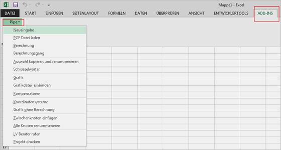
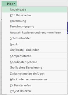
PIPE - submenu |
||
|
1. |
New entry |
Create a new project |
|
2. |
Load version 3.1 file |
Loading a project from the DOS version |
|
3. |
Calculation |
Starting the calculation |
|
4. |
Calculation process |
Displays the calculation process after a calculation |
|
5. |
Copy and renumber selection |
Copies the selected lines and pastes them behind the selection with renumbered nodes. |
|
6. |
Keywords |
Displays the help for the keywords |
|
7. |
Graphic |
Display the graphic with all options |
|
8. |
Embed graphic file |
Creates a copy of the desired graphic in the document |
|
9. |
Expansion joints |
Table for the design or selection of expansion joints |
|
10. |
Coordinate systems |
Setting the coordinate system |
|
11. |
Graphic without calculation |
Shows the graph based on the entered coordinates |
|
12. |
LV consultant call |
Starts Teamviewer remote maintenance |
|
13. |
Print project |
Especially from Office 2010 - printing process is prepared, sheets are formatted. |
|
The program is activated via the menu item "Pipe" and "New entry". or over loading a saved Excel workbook with a pipe problem.
After the start you have three tables at your disposal |
|
The project table can be found under the table name "Project". In this table the general project data and calculation options are defined.
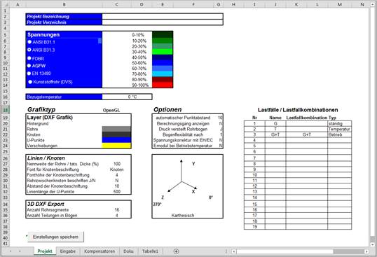
Project name, variant, revision etc. can be entered here for documentation. Together with the Excel internal options like footer and header you can design your individual calculation documentation.
This option is used to select the calculation rules for the stress calculation and for the display in the graph.
Stress determination according to
1. ANSI B 31.1 Piping in power plant applications
2. ANSI B 31.3 Piping in chemical plant construction
3. FDBR Piping calculations according to the FDBR professional association
4. AGFW district heating pipelines (chargeable add-on)
5. EN13480 Metallic industrial piping
6. Plastic pipe (DVS)
Division of the voltage range into 10 areas with color assignment. The ranges refer to the permissible voltage as a percentage or, if this is not available, to the maximum occurring voltage. Only use standard colors for the color coding!
Reference temperature is also called installation or assembly temperature. Based on this temperature and the calculation temperature (see keyword "Temp"), the temperature difference for the longitudinal expansion of the pipeline is determined.
The reference temperature can be changed with the keyword "AMBIENT =" within the pipe run. The change is valid until the next change of the reference temperature.
Settings for calculations and handling
Automatic point spacing
This option determines whether (value > 0) and at what interval the program sets the label for the next calculation point.
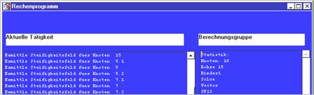
Display calculation course
During the calculation of the pipe system, the actual calculation module briefly documents the progress of the calculation. This calculation documentation can be greatly extended with this option. The option can be used especially for error analysis.
Pressure stiffened pipe bend [J / N].
The internal pressure has a stiffening effect due to the different sheet lengths of the inside and outside. This is particularly noticeable at higher pressures and can be taken into account with this option.
Sheet flexibility according to (if different from the specifications of the selected standard)
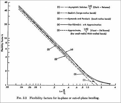
This option sets the calculation of the sheet flexibility. You can choose from 5 options suggested by the program. The calculation rules mentioned above fall back on the first option.
Side note
For the calculation of spatial pipelines,
the behavior of the bends has the decisive
influence!
Unfortunately, the behavior of an arc cannot be mapped, or only with extremely high mathematical effort. For this reason, substitute systems were sought at an early stage that would keep the computational effort within reasonable limits. A straight pipe was selected as a substitute system, to which a flexibility factor was added. This factor describes how much more flexible a bend behaves compared to a straight pipe.
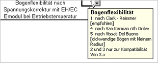
(see D. Fischer, "Rohrleitungstechnik", Vulkan Verlag, 1999, page 24ff).
Overview sheet flexibility
Voltage correction with EH / EC
This option corrects the calculated stresses in the ratio of the elasticity moduli.
>> This option should not be used with the above calculation rules.
Emodule at operating temperature
With this option, the temperature load case is calculated with the "softer" Emodulus at operating temperature, resulting in lower stresses.
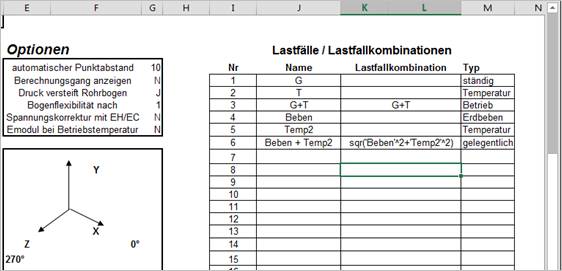
Here you can define additional load cases and load case combinations. You specify the type of combination in the Load case combination case. As a rule, this is a simple signed addition. However, depending on the set of rules, an addition with absolute values can also be formed
e.g. Quake+Temp2= ABS('Quake'+'Temp2').
VB Scripting for mathematical functions is integrated.
Hint:
· The load cases must be set in quotation marks (').
· A space must be placed before the 1st apostrophe!
· The first three load cases (G, T, G+T) are preset by the program and cannot be changed.
The load cases and their combinations are created in the input table. The boundary conditions are specified there.
Load combinations can be formed according to different rules. These rules are documented in the national regulations. Usually, a load case is formed by pure addition. An example of this is the standard combination load case of weight and temperature G+T.
However, the absolute amounts of the load cases can also be added, e.g. ABS('G')+ABS('T').
Common is also the SQSS superposition (Square root of sum of squares) e.g. SQR('G'^2+'T'^2)
Also conceivable are factors in the superposition e.g. 1.6*'G'+'T'.
In this options block the settings for the DXF (AutoCad) graphic are defined.
|
1. Layer.
2. Lines / Nodes Here you will find the settings for the display of the pipeline, the auxiliary lines and the node labeling. Representation of the pipeline thickness to the existing nominal width. The more complex the system is, the smaller the selected value should be.
3. Font and font height for the caption
4. Display and labeling of the pipe bend intermediate nodes. A pipe bend consists of 3 nodes. 5. Line length for labeling. Distance to the pipeline 6. Line length of the representation support points |
|
This option sets the 3D DXF settings.
1. Number of pipe segments: Number of corners of a polygon through which a circle is replaced.
2. Number of bend segments: Number of straight pipe segments, as a replacement for bends.
|
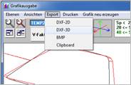
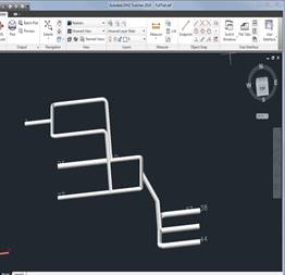
If a DXF file is displayed via PIPE - Grafi, this file can be exported in the graphic output and opened in an external viewer or in AutoCad. |
|
In this table the definition of the problem is made. The table consists of seven columns, which are used to describe the internal and external geometry, the boundary conditions and the loads,
as well as other freely definable load cases and load case combinations.

For handling, please refer to the corresponding chapters.
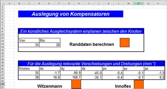
A separate calculation table with interfaces to programs of the expansion joint manufacturers has been incorporated to take artificial expansion compensation into account. Integrated Witzenmann (Flexperte version 2.0) and Innoflex database for expansion joints.
Procedure
An expansion compensation is to be installed in a pipe section between the start node 10 and the end node 20. The start and end nodes are first entered in the "From" and "To" columns. The boundary conditions for this pipe section or for the design of a compensation system are determined using the "Calculate boundary data" button.
The calculation program now determines an unobstructed line movement between these nodes. These displacements and twists are to be compensated by an artificial compensation system. (see Compensators)
|
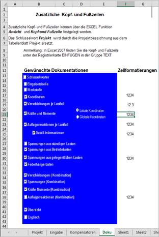
This table is used to define which information is to appear in the documentation or which additional project data is to be included in the document. The header and footer set here will be adopted for the entire project.
The Project keyword is replaced by the project name from the Project worksheet. Under Cell formatting you specify the desired format of the number representation for the respective selected result table separately. |
|
|
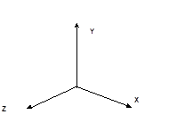
For the coordinate system, the following agreement applies first:
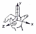
This coordinate system corresponds to the 3-finger rule of the right hand and denotes the standard coordinate system.
|
|
|
|
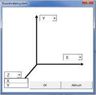
This system can be freely defined in the project table: |
|
|
|
|
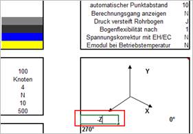
Conditions that occur at points, such as supports and external forces, can only occur at a defined node. Only at a node can a line characteristic change, only at defined nodes can forces be introduced and removed. The position of the nodes is uniquely defined by a corresponding vector in space, thus the position of each element in space is also uniquely defined.
In order to be able to process a problem, the problem must be described to the calculation program. This description takes place over a common language with defined vocabulary and with an own grammar. This makes the communication possible of the user with the computation program over the problem.
Notice:
The vocabulary or keywords describe certain properties and conditions . It is useful, but not necessary, to use the keywords in the line to which they refer.
Important:
Only one keyword of the same type is interpreted per line. e.g.
RES(30)=X RES(40)=Y.
In this case the 2nd keyword RES(40) is ignored.
|
Description of the keywords of the input |
|
|
!!xxx!! |
Comment on the calculation. Everything written between two exclamation marks is interpreted as a comment. |
|
AMBIENT=Z |
Ambient temperature Z [°C] The new reference temperature Z applies from this point. |
|
ANC(P) |
Fixed point at point P |
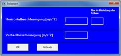
|
BEBEN_H |
Horizontal earthquake load in both directions |
|
BEBEN_V |
Vertical earthquake load |
|
BEBENXH |
Horizontal earthquake load in X-direction only |
|
BEBENZH |
Horizontal earthquake load in Z-direction only |
|
BOGWS=Z |
Additional wall thickness Z [mm] in the bend area |
|
BWT |
Weldolet (branch welded-on tea) |
|
CF |
Wind coefficient for wind loads |
|
CG x= y= z= |
Center of gravity of a valve with the position (x/y/z) related to the center of the pipe section. Only in conjunction with WEI. |
|
CONTO(P) |
Support point is connected to another node (P) of the pipeline (console support) |
|
DEL(P)Y=Z |
Displacement at point P in direction Y by Z [mm]. Directional data in the global coordinate system! |
|
EMOD=Z |
E-modulus [N/mm²] |
|
EXP |
Input of the expansion coefficient in [10^6 1/°C]. |
|
FDK=Z |
Spring constant Z [N/mm] |
|
SPRING(P) |
Spring at point P |
|
FLA |
Guide bearing (axial) in BIS node |
|
Flange |
Calculates the flange load with LV modules taking into account the current pipeline load |
|
FLEXCA=Z |
Bending compensator with spring constant Z [N/mm]. |
|
FLEXCX=Z |
Axial expansion joint with spring constant Z [N/mm]. |
|
FLEXKA=Z |
Cardan joint with spring constant Z [N/Grd] |
|
//FLEX |
Any components can be described with this keyword. It is recommended to enter the data via the input help. |
|
FLEXLN=Z |
Universal lateral expansion joint with spring constant Z [N/mm]. |
|
FLEXLX=Z |
Lateral compensator with spring constant Z [N/mm] Bending about X |
Description of the keywords of the input |
|
|
FLEXLY=Z |
Lateral compensator with spring constant Z [N/mm] Bending about Y |
|
FLEXLZ=Z |
Lateral compensator with spring constant Z [N/mm] Bending about Z |
|
FLEXTX=Z |
Angular compensator/knee piece with spring constant Z [N/Grd] Bending about X See example angular compensators (FLEXT) |
|
FLEXTY=Z |
Angular compensator/knee piece with spring constant Z [N/Grd] Bending about Y See example angular compensators (FLEXT) |
|
FLEXTZ=Z |
Angular compensator / elbow with spring constant Z [N/Grd] Bending about Z See example angular compensators (FLEXT) |
|
FLFO=Z |
Additional axial force Z [N] for non-pressure-relieved expansion joints |
|
FOR(P)Y=Z |
Global force at point P in direction Y with magnitude Z [N]. |
|
FRIC(P)=Z |
Bearing friction at point P with coefficient of friction Z |
|
GAP(P)Y=Z |
Bearing clearance at point P in direction Y by amount Z [mm]. |
|
HAG |
Height above ground in [m] for wind loads |
|
IFOR=Z |
Preload force of a spring by Z [N] |
|
K= |
Input of the k-value for occasional loads according to B31.1 104.8.2 Formula 16 (1.15 or 1.2) |
|
KO |
Coordinate definition of the starting point |
|
CONST |
Design of a constant hanger |
|
KORR=Z |
Indication of corrosion / wall thickness undercut [mm]. |
|
LifeC=X |
Number of startup and shutdown cycles |
|
MAT=Z.ZZZZ |
Material key (E-modulus and elongation are taken from the internal material data file) |
|
MAXSIF=X |
Maximum stress increase factor X (only for plastic pipes) |
|
MOM(P)Y=Z |
Global moment at point P around Y with magnitude Z [Nm]. |
|
MSIF=X |
Sets the stress increase factor X |
|
NAHT |
Consideration of stress increases due to different wall thicknesses and weld seam designs |
|
NAME='XX' |
Designates a bearing |
|
NOPIPE |
Specifies that the pipe section from the "FROM" to "TO" node is not treated as a pipeline and is not displayed graphically (thin rubber rope). NOPIPE describes the corresponding section as a 'rubber band' i.e. no pipeline exists between the initial nodes and final nodes. The keyword can be used to 'break up' a complex system to analyze the subsystems. |
|
NUE= X |
Set a transverse contraction number (Poisson's ratio) different from the database. |
|
NW=Z |
Tube outer diameter Z [mm] |
|
PRES=Z |
Internal system pressure Z [bar] / gauge pressure |
|
REDU |
Specification of a reducer for nominal size change |
|
REL(A) |
To design the spring in the weight load case, release anchor A in the direction of the weight. |
|
RES(P)=X,Y |
Obstruction at point P direction X and Y |
|
RFT Z |
Reinforced tee, Z [mm] thick reinforcing washer |
|
RIGID |
Bending resistant element |
|
RED(P)=Y |
Rotation stop at point P around Y |
|
SC=X |
Permissible stress in the installed condition in [N/mm²]. |
|
SEGB=X |
Segmental arc, where X is the pitch angle in [Grd]. |
|
SH=X |
Permissible stress at maximum temperature in [N/mm²]. |
Description of the keywords of the input |
|
|
SLASTX=Z |
Line load in direction X with magnitude Z [N/m]. |
|
SLASTY=Z |
Line load in direction Y with magnitude Z [N/m]. |
|
SLASTZ=Z |
Line load in direction Z with magnitude Z [N/m]. |
|
SPT=X |
Special tee where the user can enter the stress increase factor (SIF) himself X = SIF |
|
ST=X |
Yield strength at room temperature in [N/mm²]. |
|
STABIL |
Stability verification according to 18T4 or Eurocode 8 with LV modules see example stability calculation (STABIL) |
|
Socket |
FEM calculation with LV module for nozzle connections |
|
TEMP=Z |
System temperature Z [°C] |
|
TYPICAL name [ TYPICAL name ] |
Defines a typically recurring pipeline element or component. The name can be freely selected. See description of keywords |
|
UFT |
Unreinforced tee |
|
UNIF=Z |
Line load Z [N/m] |
|
VS(P)=Z |
Preload of Z [mm] applied at point P |
|
WEI=Z |
Special load Z [N] |
|
WIND=A |
Wind load according to DIN 1055 from direction A (+X, -X, +Y, -Y) |
|
WINDq=X |
Dynamic pressure x in [kN/m²] , if different from DIN 1055 |
|
WLT |
Welded tee |
|
WS=Z |
Pipe wall thickness Z [mm] |
|
Column R |
R=radius: it corresponds to S=3D and L=5D arc or direct input of the radius [mm], arcs and radii refer to the next change of direction, i.e. to the BIS node. NW,WS,MAT,UNIF,TEMP are valid from VON node |
|
Description of the output keywords |
|
|
Sa |
Equivalent stress at the beginning of the pipe in the local system |
|
Se |
Equivalent stress at the pipe end in the local system |
|
Sla |
Longitudinal stress at the beginning of the pipe |
|
Sle |
Longitudinal stress at the end of the tube |
The following keywords are available for entering the external conditions:
TEMP =, UNIF =, PRES =, WEI =, DEL (), FOR (), MOM (), SIF () and MSIF
All
entries are made in the Additional data column. The order is
irrelevant.
Upper/lower case is not distinguished, i.e. TEMP = is identical with temp=.
All data refer to the VON node unless explicitly stated.
|
Keywords |
|
|
TEMP = |
Entering the operating temperature (Calculation temperature, also minus temperatures allowed TEMP= -35).
Example: TEMP =320From |
|
UNIF = |
Input of the line weight of a pipeline incl. insulation ice and water load in [N/m].
Example: UNIF=400From |
|
PRES = |
Input of the calculation pressure in bar / gauge pressure This applies to the entire piping system. |
|
WEI= |
Input of an additional concentrated load in N This
engages in the middle of the pipe section and is used, for example, to
account for fittings. Example: WEI =2000 A weight force of 2000 N acts in the middle of the pipe section between the VON and BIS nodes. |
|
CG x=a mm y=b mm z=c mm |
Input of a center of gravity of a valve deviating from the center of the pipe section Applies only in conjunction with HOW Example: CG x=20 y=0 z=50 The center of gravity of the valve deviates from the center of the pipe section. It is located in space 20mm in X-direction 0mm in Y-direction and 50mm in Z-direction from the center of the pipe section. Input of coordinates Global! |
DEL (X)Y=Z |
Forced displacement of a node for the temperature load case Example Input: DEL
The direction information refers to the global system! The keyword DEL always refers to the temperature load case only, unless it is forcibly assigned to the weight load case with the keyword LF=1 (load case=1 = weight load case). |
|
FOR (A)B=C |
Input of an additional force at node A in N. The force acts in the global direction B
Example: FOR The keyword FOR refers only to the weight load case, unless
it is forcibly attributed to the temperature load case with the
keyword LF(load case=2 = temperature load case). FOR cannot be used in supports with obstruction in the direction of force. |
|
Keywords |
|
|
MOM (A)B=C |
Input of an additional moment in node A with the amount C in N/m. The moment acts around the global axis B (X, Y or Z). Example: MOM(47)Y=2345 Annotation: The direction specifications refer to the global system!
|
|
VS =C |
Input of a prestress in the pipe section with C mm
Example: VS =20 Annotation: The preload can only be applied at an axially fixed bearing point and in front of the point at which it is to act
|
|
SlastX=C |
Input of a line load with the magnitude C in N/m in direction X Example: SlastX=100This |
|
SlastY=C |
Input of a line load with the magnitude C in N/m in direction Y Example: SlastY=100This |
|
SlastZ=C |
Input of a line load with the magnitude C in N/m in direction Z Example: SlastZ=100This To enter the pipe dimensions you can use the keywords |
|
NW= |
Enter the outer diameter of the pipeline in mm. The entry is valid from the VON node until it is overwritten by a new entry. Example: NW=114.3 |
|
WS= |
Enter the wall thickness in mm Example: WS =6.3 |
SEGB=X |
denotes a segmental arc, where X is the pitch angle in Grd. Example: A Radius 2000 Special data SEGB=22.5 |
|
Keywords |
|
|
SSEGB=X |
Designates a segmental arch with only one intermediate piece |
|
BogWS = |
Enter the wall thickness in mm. The input is valid from the VON node until it is overwritten by a new input.
This means that all bottom wall thicknesses are 3 mm smaller than the pipe wall thicknesses specified with WS =. This entry is valid until it is overwritten by another entry. |
|
KORR =X |
Indication of corrosion or wall thickness undercut. Example: Corr=1.5 This means that the wall thickness in service can be up to 1.5 mm less than in the installed condition. The flexibility of the pipeline is determined with the stiff, non-corroded pipeline, the occurring stresses are related to the corroded wall cross-section. This entry is valid until it is overwritten by another entry. |
|
WINDq=X |
Enter a dynamic pressure in kN/m² that deviates from DIN 1055. |
|
RIGID |
Between the VON
and BIS nodes there is a rigid element, e.g. a fitting. This affects
the movement of the pipeline. |
|
SIF (A)=X |
A stress increase factor of X is defined at node A. An input smaller than 1 is corrected to 1 by the program. |
|
MSIF =X |
For the whole piping system from this input the This is valid until it is overwritten by another input from MSIF. An input smaller than 1 is corrected to 1 by the program. |
|
TYPICAL name ] |
Defines a typically recurring pipeline element or component. The name can be freely selected. The number of nodes in the typical element must be taken into account when assigning the FROM and TO nodes. The typical element can be used basically everywhere and is specified by 'Typical' plus the assigned name. Example:
|
|
AMBIENT = Z |
Change in ambient temperature / reference temperature [°C]. The input is valid from the VON node until it is overwritten by a new input. |
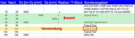
Description of the keywords MAT, MATID, EMOD, EMODC, EXP, . POISSON , SH , SC , ST , LIFEC
|
Keywords |
|
|
EMOD= |
Input of the E-modulus N/mm2 This entry refers to the VON node and is valid until the next entry. Example: EMOD =200000 |
|
EMODC= |
Input of the E-modulus N/mm2 at installation temperature This entry refers to the VON node and is valid until the next entry. Beispiel: EMODC=206000 |
|
EXP = |
Input of the expansion coefficient in 10Ù6 mm / °C This specification is valid from the VON node to the next entry. Example: EXP =12.3 Since you also receive a material database with the PIPE program, you can also obtain information on the piping material directly from the database. The input of the Young's modulus and the expansion coefficient can therefore be replaced by the specification. |
|
MAT = |
Input of the material type This input is also valid from the VON node until it is modified by a new input. Example: MAT =F (ferrite) or MAT=A (austenite) IMPORTANT: |
|
SH =XXX |
Permissible stress at maximum temperature in N/mm2 |
|
SC =XXX |
Permissible stress in the installed condition in N/mm2 |
|
ST =XXX |
Yield strength at room temperature in N/mm² |
|
LifeC=X |
Number of startup and shutdown cycles |
|
NUE= X |
Set a
transverse contraction number |
|
MatID=X |
Specification of the identification number of the material database |
|
K= |
Input of the k-value for occasional loads according to B31.1 104.8.2 Formula 16 (1.15 or 1.2) |
|
Keywords |
|
|
FLEXCX=X |
Spring constant in N/mmfor axial expansion joint |
|
FLEXCA=X |
Spring constant in N/mm for bending compensator |
|
FLEXLX=X |
Spring constant in N/mm Lateral compensator Bending around X axis |
|
FLEXLY=X |
Spring constant in N/mm Lateral compensator Bending around Y axis |
|
FLEXLZ=X |
Spring constant in N/mm Lateral compensator Bending about Z axis |
|
FLEXLN=X |
Spring constant in N/mm Universal lateral compensator |
|
FLEXTX=X |
Spring constant in N/Grd Angular compensator/knee piece Bending around X axis |
|
FLEXTY=X |
Spring constant in N/Grd Angular compensator/knee piece Bending around Y axis |
|
FLEXTZ=X |
Spring constant in N/Grd Angular compensator/knee piece Bending about Z axis |
|
FLEXKA=X |
Spring constant in N/Grd Cardan joint |
|
FLFO=X |
Additional axial force Z [N] for non-pressure-relieved expansion joints |
Expansion joints should be calculated without friction to avoid uncontrolled movements.
Adjustment rate K specified by the manufacturer in [Nm / °].
K Nm must be applied to rotate the compensator by 1°.
With the compensator length L follows
z. e. g. length L = 350 mm

a displacement at the compensator end
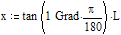
and thus a spring constant of


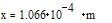


corresponds to 6.449^*10^7 N/m or 6.449*10^4 N/mm
For the support of a pipeline there are several basic types of fasteners, e.g.
· Fixed points without degree of freedom,
· Linear obstructions such as supports and stops,
· variable suspensions via springs
· non-linear supports such as supports with friction or support play.
The keywords used to describe all these variants are listed below.
|
Keywords |
|
|
ANC (A) |
At node A there is a fixed point (anchor) Example ANC |
|
RES (A)=B |
Sliding bearing in node A. Direction B (X, Y or Z) is restrained. ExampleA RES |
|
RED (A)=B |
Rotation stop at node A around axis B (X, Y or Z). This type of support stops the rotation of the pipeline around any axis of coordination. Example |
|
FLA |
Guide bearing at the BIS node. This keyword designates a guide bearing with locked weight direction and lateral guidance. It is particularly suitable for simulating inclined guide bearings, i.e. guide bearings for pipelines which are not parallel to a coordinate axis. NOTICE: If a guide bearing is to be provided with clearance, the keyword RES must be used! FLA cannot be combined with GAP! |
With the LV-Pipe II program, both spring hangers can be simulated and designed.
|
Keywords |
|
|
SPRING(A) |
Example: If the keyword FDK (spring constant) is used subsequently to this input, the spring is simulated at point A. If no entry is made for the spring constant, the spring is designed at point A. The program calculates a spring constant so that the difference between the mounting and operating load on the spring is less than or equal to 10%. This requires a calculation of the entire system twice |
|
FDK |
Specification of a spring constant in N/mm for a known spring Example: SPRING (67)FDK =200At |
|
FDW=x |
The spring hanger is selected so that there is a difference of x% between the load case weight and the combination load case temperature + weight Example: SPRING (67)FDW |
|
IFOR |
Specification of a preload for a spring i.e. the spring is preloaded with a force (N) during assembly. Example: FEDER (67)FDK =200 IFOR =100 The spring at node 67 should be preloaded with a force of 100 N |
|
CONST |
Spring is defined as a constant hanger. Example: FEDER(67)KONST AM node 67, a constant hanger is determined that takes the load from the pure weight load case G, independent of the line movement for all load cases. |
|
LISEGA |
Using the Lisega catalog for spring selection |
|
HYDRA |
Using the Hydra catalog for spring selection |
|
REL (A) |
For the design of the spring in the weight load case: Armature A is released or unloaded in the weight direction in order to achieve a stress-free installation. Example: REL |
|
Keywords |
|
|
//FLEXComponent |
Any components can be described with this keyword. It is recommended to enter the data via the input help. |
|
Keywords |
|
|
NAME='example' |
Bearings can be named with this keyword. This name is listed in the documentation Example: ANC |
You can use the keywords GAP and FRIC to describe special support conditions.
|
Keywords |
|
|
GAPX=A GAPY=A GAPZ=Y |
Bearing clearance in direction X, Y and Z by A mm. This means that a pipeline can move A mm before movement in one direction is impeded |
|
Example: RES (43)=X |
|
|
FRIC=B |
The displacements are hindered by friction with the coefficient of friction B Example: The movement is hindered by a coefficient of friction of 0.56. The
coefficient of friction is understood as the proportion of the forces that
counteract the movement. It depends on the surface condition of the bearing
elements. |
|
FR =B |
The displacements of the support defined shortly before are hindered by a friction with the coefficient of friction B Example: Res(80)=Y FR=0 This means that the friction set globally with the FRIC keyword is removed for the support 80 (hanger). |
Pipe bends and tees can be defined in the input fields with the heading R.
S designates a 3D sheet. The DIN is deposited and is activated in the relevant case.
L designates a 5D sheet. The DIN is deposited and is activated in the relevant case.
Any number X creates an arc with radius X (in mm).
BWT designates a Weldolet (branch welded-on)
WLT designates a welded T-piece or normal fitting
UFT designates an unreinforced T-piece
RFT =Xdenotes a reinforced tee, where the reinforcing washer is X mm thick.
SPT=X designates a special tee where the user can enter the stress increase factor (SIF) himself. SPT can be used instead of BWT, WLT, UFT or RFT.
Ex: SPT = 1.3
The coordinates of a point can be specified with the KO keyword.
Syntax:
From = node name
After = KO(keyword)
Dx,Dy,Dz = absolute coordinates of the point
Notice:
KO must not be used in the first line!

Keywords are entered in the "Special data" column, with the exception of arcs and tees.
The KO keyword is used in the "AFTER" column.
The program is not case sensitive:
RES (45)=X is equivalent to Res(45)=x. However, the notation must be observed, this also applies to the blanks.
Descriptions that cannot be interpreted are considered comments.
Example:

Keywords can be entered directly into the corresponding columns or modified there.
Since descriptions that cannot be interpreted are comments, a small modification allows the calculation to be performed with alternatives.
If you want to execute the calculation without the spring in the above example, it is sufficient to change the keyword SPRING (17) to FXDER(17). It will no longer be recognized by the program as a keyword and will be treated as a comment.
>> A simple change of the X to an e activates the spring again.
So that not all entries have to be typed in, an input help can also be activated in Excel. This is done by double-clicking in the Special data column.
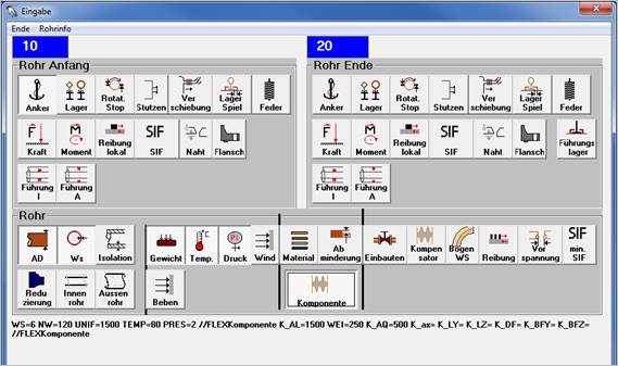
The blue fields (10) and (20) contain the nodes at the beginning and end of the section. For each of these nodes, corresponding node information can be selected from the "Pipe start" or "Pipe end" frame. Details of the pipeline between the nodes are selected from the "Pipe" frame. The selected indications are represented by the color marking of the buttons, moreover, the keywords are displayed according to the selection. By clicking the button again, the entries can be modified or deleted. The OK button confirms the entries, the Cancel button discards them.
Some buttons call up another input form to request further information.
These additional forms are tabulated below.
Button |
Additional form |
Description |
|
|
|
Fixed point No pipeline movements and rotations possible |
|
or
|
|
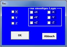
Determination of the obstruction in direction X,Y and / or Z or the rotation around X,Y and / or Z either in positive and negative direction or in one direction of the axis
|


Button |
Additional form |
Description |
|
|
|
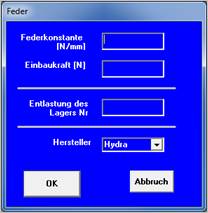
Defining the additional keywords to the spring keyword.
FDK ;IFOR ; REL (); Lisega and Hydra. All entries are optional.
See corresponding keyword description. |
|
or
or
or
|
|
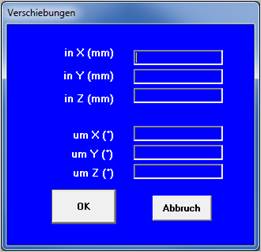
Defines bearing movements or bearing rotations in X,Y and / or Z. Unit mm or degrees.
Defines an external force in direction X,Y and / or Z. Unit N
Defines an external moment around X,Y and / or Z. Unit N/m.
Defines the bearing clearance in the obstruction direction X,Y and / or Z. Unit mm. |
|
or
|
|
Defines the coefficient of friction
global or local
|
|
or
|
|
Defines
the stress increas
local or global |





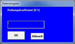


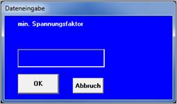
Button |
Additional form |
Description |
|
|
|
Input of the pipe outer diameter. Unit mm |
|
|
|
Input of the wall thickness. Unit mm
|
|
|
|
Input of the calculation temperature.
Unit °C.
|
|
|
|
Input calculation pressure unit bar(g) / gauge pressure |
|
|
|
Input of all reductions such as corrosion and wall thickness undercut.
|

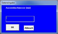

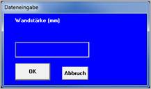

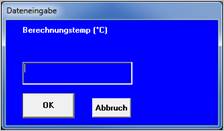

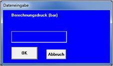

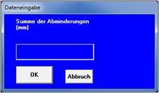
Button |
Additional form |
Description |
|
|
|
|
Input of fittings etc.
|
|
|
|
|
|
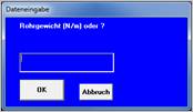
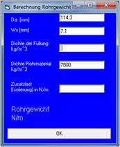
Input of the pipe weight.
Entering a question mark opens the calculation form for the pipe weight.
|
|
|
|
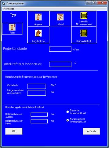
Generation of compensator keywords.
Deposited manufacturer catalogs
Calculation of the spring constants from the adjustment rate.
Calculation of the additional axial force (see FLFO short description of keywords). |
|

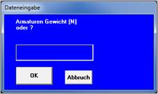


Button |
Additional form |
Description |
|
|
|
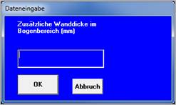
Input of the thickness difference pipe bend to straight pipe.
|
|
|
|
Consideration of preload
|
|
|
|
Consideration of |
|
|
|
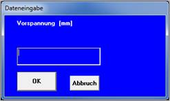
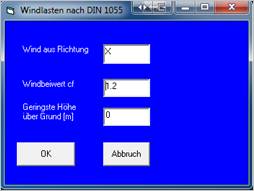
Consideration of wind loads according to DIN 1055 with 'lowest height above ground the starting height of the pipeline can be defined.
This input must be made only once. The dynamic pressure is calculated according to DIN 1055.
If another value is to be specified, this can be done with this keyword WINDq = X |




Button |
Additional form |
Description |
|
|
|
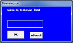
Consideration of insulation thickness only for wind load calculation |
|
|
|
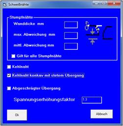
Consideration of Stress increases due to different wall thicknesses and weld designs. |
|
|
|
Guide bearing. Obstruction of weight and normal movement. |
|
|
|
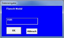
Calculates the flange load taking into account the current pipe load. This option is only active if the corresponding LV module for flange calculation has been purchased or is available via FEEZING. (Modules for flange calculation: 25V, B8, 1591, AFL) |




Button |
Additional form |
Description |
|
|
|
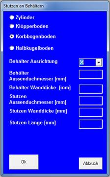
Calculation of nozzle connections on vessels.
This option is only active if the FEM (Finite Elements) module has been purchased or is available via FEEZING (see ATLAS manual). |
|
|
|
Reductions are taken into account in the stress evaluation or only in the graphical representation, depending on the regulation |
|
|
|
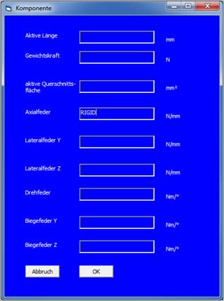
Input of any pipe components. Stiffness can be specified with 'RIGID' in the input form
Ex: K_AL= WEI= K_AQ= K_ax=RIGID K_LY= K_LZ= K_DF= K_BFY= K_BFZ= |



|
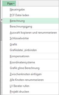
The calculation is started via the menu item "Pipe" and "Calculation".
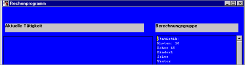
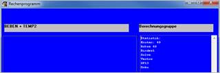
Display during calculation
During the calculation the calculation progress is documented. This documentation can be controlled by the option "Show calculation progress" in the project sheet (see above).
|
|
|
|
|
|
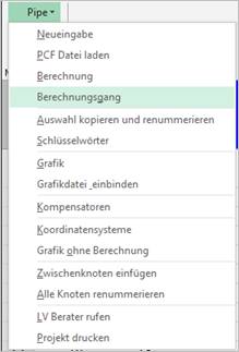
The display can also be called up again after the calculation has been carried out by means of the menu item "Pipe" and "Calculation course".
|
|
Control of the scope of documentation
Tables to be created in the documentation can be selected in the Docu table.
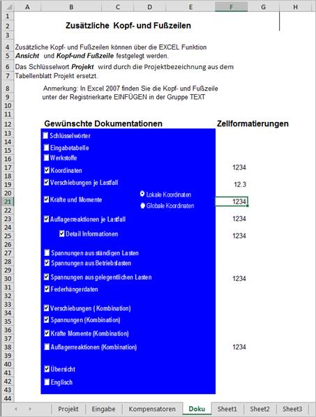
In this table you can also define the headers and footers of the project.
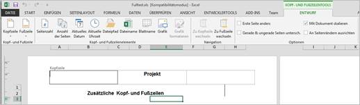
|
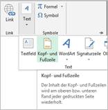
Select in In Excel 2007/2010: "Page Layout" and then "Page Setup", "Header and Footer".
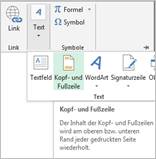
In EXCEL 2013/2016 "Insert" and then "Text", "Header and Footer".
|
|
After the calculation is completed, the LV program creates a new workbook with the following tables:
|
Input table |
The input table can be output for documentation purposes. The input table is inactive in the documentation folder. |
|
Keywords |
Table with explanations of the keywords of the input table |
|
Materials |
Table with the material data |
|
Display of the calculated pipeline movements separately for the load case weight and temperaturein the global system |
|
|
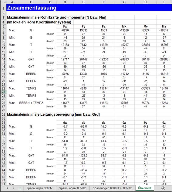
Display of the calculated internal pipe forces and moments In the local system, i.e. the X-axis is the pipe axis. The pipe is cut free and the forces are calculated. If there is no change in direction, the forces before and after the intersection point are equal, but have opposite signs. |
|
|
Display of the support load separately for weight and temperature load case |
|
|
Voltages G |
|
|
Tensions T |
|
|
Display of the calculated internal piping forces and moments for the combination load case |
|
|
Tensions |
Weight + Earthquake + Wind |
|
Overview table |
Summary of the main calculation results |
The program automatically gives a name to the newly created workbook. Possibly, the existence of a workbook with the same name is pointed out. With this procedure, calculation results can also be loaded independently of the input file.
If your computer has an OpenGL capable
graphics card, you can use the advanced graphics options.
In the project window, select the OpenGL graphics type.
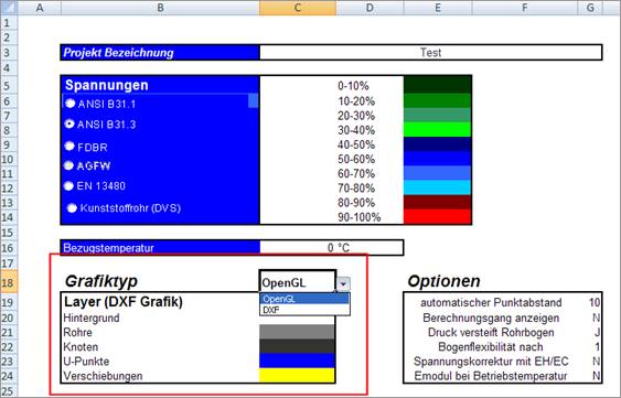
If the graphic type is changed, this only becomes active after a recalculation, since the calculation module also generates the necessary data for the display, among other things.
If a recalculation was carried out
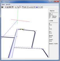
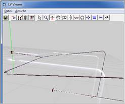
successfully, a 3D graphic of your system can be displayed via the Graphic
option in the Pipe menu.
3D graphic of your system can be displayed.
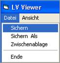
Under the "File" menu you can save the currently displayed graphic in bitmap (BMP) format. The saving is done either to the last file name or with the option "Save as" to a new file. With the submenu "End" the viewer can be terminated.
|
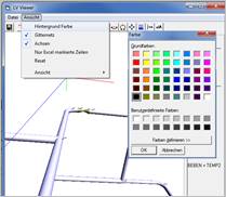
Freely selectable color for the background of the graphic display
|
|
|
Fades the grid in and out.
|
|
|
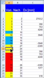
Mark the nodes you want to display in the graphic in the input sheet with any background color. This allows you to represent non-contiguous pipelines and areas. Select a cell. All cells in the same color are now displayed in the viewer.
|
|
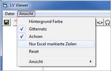
This option performs a complete rebuild of the graphic.
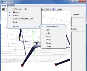
Here you have the possibility to switch between standard views.
The representations in detail
|
|
|
|
|
Perspective |
Above |
Links |
|
|
|
|
|
Front |
Below |
Right |
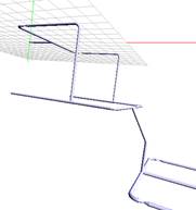
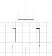
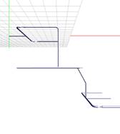
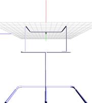
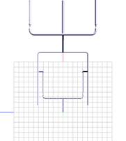
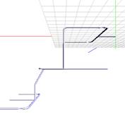
Not shown is the "Rear" view
|
Unscaled representation, to shorten long pipelines:
|
|
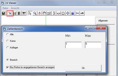
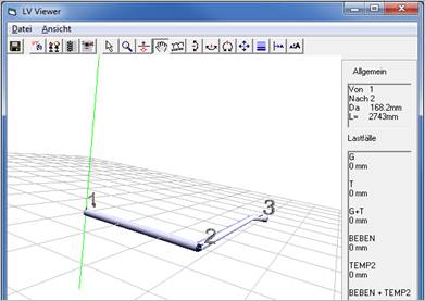
Display nodes and pipelines in a specified number range.
Other pipelines are hidden:
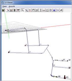
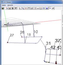
To avoid confusing displays, the spacing of the node designation as well as the font size can be freely selected.

|
Before
|
After
|
With the icon / button bar you can reach more options faster.
Button |
Description |
|
|
|
Save the current view (see menu) |
|
|
|
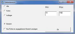
This option shows the node names. If this button is pressed, another selection menu appears. In this form you can define whether all nodes or only a node range should be labeled or whether the node label should be hidden again. |
|
|
|
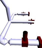
Showing and hiding the supports
Example : Fixed points, guide bearings and spring hangers inserted
|
|



Button |
Description |
|
|
|
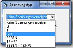
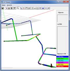
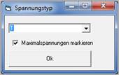
Representation of the voltages. Another selection form appears here.
In this form you define whether and for which load case or load case combination you want to display the stresses. The voltages are displayed color coded. In addition, you can display the HotSpots for each load case. The areas with the highest voltage are displayed in 'red'.
|
|
|
|
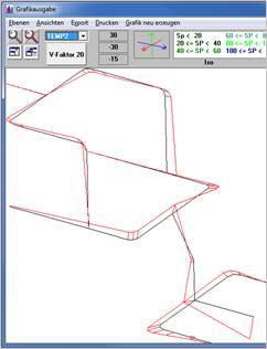
This button displays the displacements of the pipeline. Here, too, a selection form appears first. In this form, you specify whether and for which load case you want to display the displacement. The displacement can be overdrawn. This is done via the distortion factor. It can be used to represent even the smallest movements. The deformed system is shown as a thin red line, the undeformed system is drawn as a vitreous body. |
|
|
|
Animated representation of the displacement. |
|
|
|
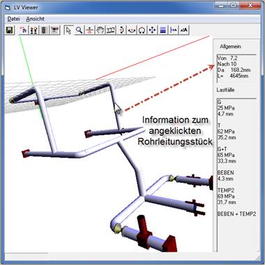
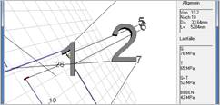
Display information about the clicked pipe string.
Individual node labels can be moved. Click on the node number in the graphic, drag the node to another position, release the mouse button and click again. |
|
|
|
Fast zoom. If this button is activated, you can zoom in (mouse movement up) or zoom out with a mouse movement down while keeping the left mouse button pressed.
|
|





Button |
Description |
|
|
Slow zoom. Handling is identical to fast zoom. |
|
|
This button allows you to move the entire view. To do this, hold down the left mouse button and move the view to the new position. |
|
|
Change the displayed pipeline size. |
|
|
Adjust the distance of the node designations from the pipeline. |
|
|
Adjust the font size of the node labels. |
|
|
Vertical, horizontal swing and rotation of the view. |


The right mouse button is used to move the entire view freely.
Hold down the right mouse button and move the view to the new position.