Voltage rating

If the normal stress σ_m of a bar made of an ideal elastic-plastic material reaches the yield point as a result of a constantly acting central normal force, its load-bearing capacity is exhausted. If the normal stress σ_b of the same bar reaches the yield point σs as a result of a constantly acting bending moment of the magnitude M_el on the outer fiber, then a load-bearing capacity reserve remains. This is until, after increasing the moment to the magnitude M_pl, a stress distribution as shown in Fig. 9.6d is achieved. The ratio

depends on the cross-section shape and is 1.5 for the rectangular cross-section.

If the bar under consideration has a notch-like change in cross-section (notch, corner), then both the effect of a central normal force and the effect of a bending moment additionally produce a normal stress σ_k with a peak-like course, which can be large but only extends over a very small cross-sectional area. The load-carrying capacity of the bar is then only impaired when, as a result of the simultaneous action of σ_m and/or σb as well as σ_k, the ultimate strain δ or the ultimate strength σ_T, is reached. Initially, only a very localized crack occurs, but it then propagates further and further with each load change.

Thus it is necessary to evaluate the stresses σ_m, σ_b and σ_k differently. In the case of the line elements to be dealt with here, the following definition is therefore agreed for the stresses distributed over the wall thickness s on the basis of Fig. 20.1

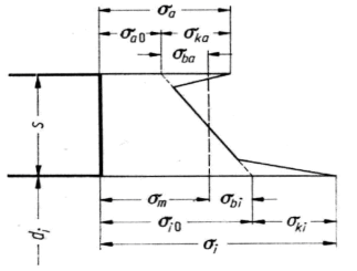
a) The membrane stress σ_m is understood to be a stress of the same magnitude and direction across the entire wall thickness. If σ_a0 and σ_i0 are given, then the following applies

b) The bending stress σb is the stress caused by a wall bending moment. If σ_a0 and σ_i0 are given, then

If the temperature at the outer wall (theta a) and inner wall (theta i) is different but linear across the wall, then it follows:

c) If σ is the total stress, then the stress peak σ_k is only the part exceeding σ_m+ σ_b, i.e.

If the total stress σ was determined via a notch or form factor σ_k to σ = σ_k - (σ_m + σ_b), then the following applies

If the voltage peak follows from a sudden heating (upper sign) or a sudden cooling (lower sign) of the outer or inner wall by delta theta, then one obtains

If a tube has a thin cladding with and E_p, then changing the assembly temperature  to the operating temperature in the cladding results in a stress peak of

If the diaphragm and bending stresses listed in 20.1 occur only in a limited area of the structure, and if, due to geometric conditions, the parts further away are then called upon to bear the load when the yield point is exceeded, then these are referred to as local stresses. In the case of cylindrical, conical and spherical hollow body parts, those membrane and bending stresses which occur within the area (from the point of their extreme value as seen in the circumferential or longitudinal direction) are usually regarded as local stresses _Lσ_.

In addition, the condition for classification as a local stress is that its extreme value is at least um away from that of another local stress. All normal and bending stresses that cannot be classified as local stresses according to these two geometric conditions are called non-local stresses _Nσ_.

For the point- or line-shaped distributed stress peaks σ_k described in 20.1, a subdivision into _Nσ_k and _Lσ_k would only have a formal meaning, since there is no difference with respect to the failure.

The essential property of a stress designated as primary stress σ^I is that it is absolutely required to establish equilibrium with respect to such external loads that continue to act in full magnitude even when the yield strength is exceeded. These external loads include

a)     Internal and external pressure

b)     All weight loads

c)     Snow and wind loads on outdoor lines

d)     Earth pressure and live load for buried pipelines

e)     Recoil forces

f)      Acceleration forces due to earthquakes

The essential characteristic of a stress called secondary stress is that it results from strains that have a limit value due to physical or geometric conditions. Secondary stresses. are thus caused by forced but limited changes in shape.

For pipelines and their elements, the following stresses fall under this term:

a)     All stresses dependent on temperature (radial and axial temperature gradient, different coefficient of thermal expansion).

b)     All stresses from prevented system longitudinal strain.

c)     All interference stresses, i.e. stresses that occur at transitions to other geometric shapes as a result of different strain behavior.

d)     All stresses which are caused by the loads listed under primary stresses, but which allow the equilibrium conditions to be fulfilled even without their presence. For example, bending stresses occur in an oval tube as a result of internal pressure. If these exceed the yield point, the tube cross-section tends toward the more favorable cylindrical shape and can absorb the internal pressure by membrane stresses. If, on the other hand, the same oval tube is under external pressure load, then the bending stress would be absolutely necessary and therefore to be regarded as primary stress.

For shear stresses caused by torsional moments or shear forces, the same subdivisions according to course (, , ) propagation (,  ) and cause apply ( , ) as for normal stresses in 20.1 to 20.3.

The definition for , , is obtained by substituting in Fig. 20.1 and in Eqs. (20.1), (20.2) and (20.5) the signreplaced by .

If you go with the abbreviations

          permissible stress K/S at temperature  due to pure tensile loading

        Yield strength at temperature

        Proportionality limit at temperature

            Equivalent stress (5.8)

from the premise

off, then applies:

If the value for a single-acting non-local primary bending stress is accepted as permissible, then a safety factor of 1.5 - 1.5/1.25 = 1.8 remains in accordance with 20.1 against failure due to yielding and no permanent strains occur.

If, on the other hand, the determined value of the bending stress is reduced to 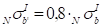,before forming the equivalent stress,    then in the evaluation of a non-local primary membrane stress           becomes equivalent.

If the value for a single-acting local primary diaphragm stress or for a single-acting reduced local primary bending stress , is allowed as a limit value, then a safety factor of 1.2 remains against yield failure for the diaphragm stress and 1.44 for the bending stress.

If the equivalent stress from the primary and secondary stresses reaches the value , then the yield strength is exceeded at the first load, but at further load changes one remains in the elastic range (because of). The reduced bending stress ab' = 0.8 - ab would therefore have to be limited to .

If this limit value is also used as a basis for the diaphragm voltages, an additional safety factor of 1.25 remains.

If the equivalent stress from the primary stresses, secondary stresses and stress peaks exceeds the value when the full magnitude bending stresses are taken into account, then an investigation for alternating stress is required.

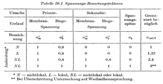
Table 20.1 summarizes the evaluation of total stresses proposed here in terms of stress evaluation factors. .

The right column indicates the multiple of the value of the

 the equivalent stress determined from the stresses multiplied by the factors on the left may increase. For the limit valuesand it is assumed that the equivalent stress is based on the entire amplitude of the individual voltages.

The evaluation of the total stresses described in 20.5 is computationally very complex, since the individual stresses must be determined once for several interfaces of the system, then there again for several cross-section points on the outer and inner wall. In most cases, this effort can be avoided for cylindrical hollow bodies by proving that subsequent limit values are not exceeded for certain individual stresses or stress sums.

(a) Equivalent stress of internal compressive stresses:

The value for is obtained by solving the respective prescribed wall thickness design formula to = K/S.

(b) Sum of the nonlocal primary longitudinal membrane voltages:

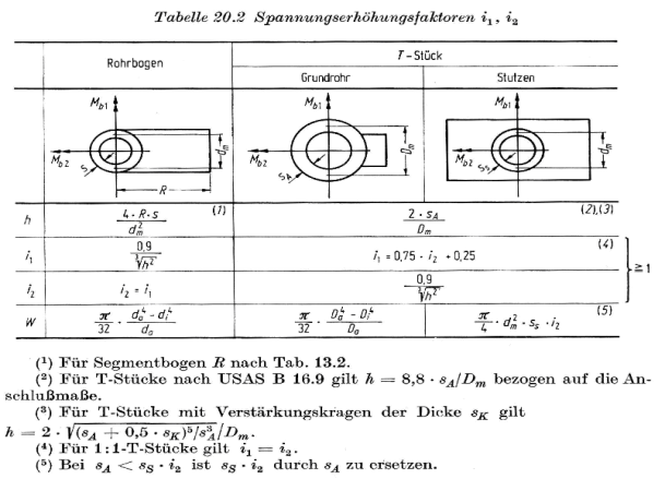
For the stress intensification factors i and section moduli W the values given in Table 20.2 apply as for c). (Cf. 11.2, 13.4, 20.1 to 20.3.)

c) Mean equivalent stress due to prevented longitudinal elongation of the system:

with

Here, the stresses for the maximum temperature difference must be determined without taking into account any prestressing.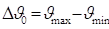

If N0 is the number of load cycles to be associated (with respect to the intended lifetime of the line) and if N1, N2 ...  Nn, are the load cycles belonging to other and smaller temperature differences , ...  then the comparative number of load cycles Nv is given by

and the corresponding factor kN

The suggestions for stress evaluation are essentially taken from the American regulations USAS B 31.1.0 to 8 and ASME Nuclear Vessels Code. In deviation from this, the factors in Tab. 20.1 were obtained by introducing the concept of reduced bending stress. This resulted in the following:

a)     Utilization of the larger load reserve for a bending stress compared to a normal force stress, but limitation of the maximum value of a non-local primary bending stress to (instead of σs).

b)     Limitation of the sum of primary and secondary diaphragm stress to (instead of ) with regard to rigidly laid cables, where the longitudinal diaphragm stresses due to temperature changes act in the same magnitude over the entire cross-section.