Unsteady calculation with the additional module KV

Unsteady calculations for incompressible mediums are done by the additional module KV. This module has to be purchased separately.

For the unsteady calculation there are following conditions:

One or more pipe runs which are directly connected to an inlet or outlet gusset with defined quantity can be linked to the module KV.

The unsteady calculation is performed for the model "Modification of a valve position". This means, that the inlet or outlet gusset, i.e. a supply or draining fitting, is modified in its valve position in a way so that a change in pressure or velocity occurs. In case of incompressible media the pressure change extends through the entire system.

After a certain time this results in a steady-state flow in the entire system.

The time course of velocity, pressure drop and volume flow in any pipe run can be recorded and be transferred to WORD for documentation or to EXCEL for further analysis.

Proceed step by step as follows:

Create the pipe network with all required gussets and pipe runs. Enter at least one inlet or outlet; the inlet or outlet quantity can be selected as you like.

Link the pipe run leading directly to an inlet or outlet gusset to the module KV in the following way:

Double-click the pipe run

Select the module KV in the pull-down list on the right

Click "Activate"

and leave the mask with OK.

Click the "Calculate" icon

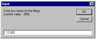
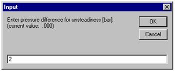
You are asked to enter the “friction factor for the (open) fitting” and the “pressure difference”. Enter the appropriate values here.

The calculation is done and the results are entered in the mask.

The volume flow in the selected inlet or outlet run has been overwritten by the calculated value.

Analyse the results of the calculation in the following way:

Select “Query time data” in the “Calculate unsteady” menu

Select “Display/print flow curve” in the “Calculate unsteady” menu

This chapter describes further possibilities which are not necessary to do simple unsteady calculations. The options described herein enable you to use a lot of further methods of analysis, e.g.:

observing the time course of any pipe run

giving any initial velocity

continuous pressure increase

saving time dependent data in WORD or EXCEL

automatic creation of a course curve as EXCEL diagram

Furthermore the extensive possibilities of the ATLAS module KV are available for you, e.g. for documentation or for parameter studies.

For the following calculations this basic model is always used:

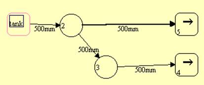
All pipes have a length of 500 m, diameter of 500 mm,

roughness 40 :m.

Pipe 3 è 4 has a fixed flow rate of 1000 l/s which has been defined via the outlet gusset 4.

All geodesic heights are 0.

The pipe drawn bold 2 è 5 has been linked to the module KV by selecting "Activate" in the input mask.

Note: Pipe runs linked to the module KV are drawn bold automatically.

For the unsteady course of the flow the following values are entered:

Friction (pressure drop) factor for the tapping-point fitting assumed to be in outlet gusset: 12

Pressure increase of 2 bar by modification of the valve position (see above) in the supply or in the entire pipe network (incompressible flow)

You can enter these values in the "Calculate unsteady" menu. If the values have not been entered they are asked automatically after starting the calculation.

In the first step of the calculation the steady-state flow rate value (more precisely: the flow rate value after reaching 99% of the end value of the unsteady process) after the pressure increase is determined and entered into the outlet gusset 5 and the pipe run:

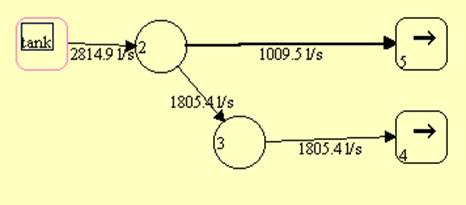
For the selected data this value is approximately 1009 l/s.

With the menu item "Calculate unsteady” – “Query time data"

the values are displayed as a function of the time:

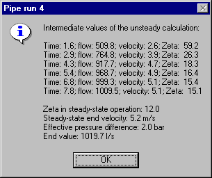
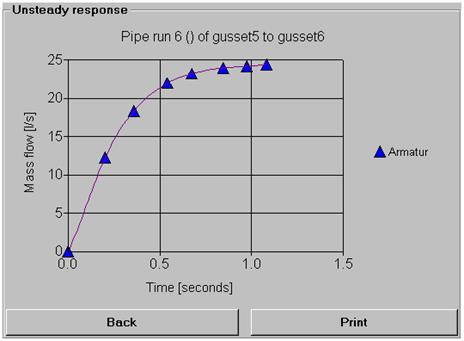
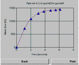
With the menu item "Calculate unsteady” – “Display/print flow curve"    the time course is represented graphically:

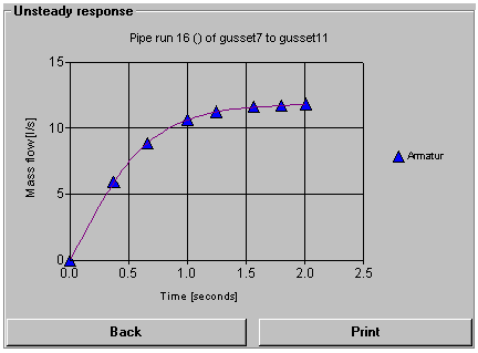
The curve can be sent to the standard printer by clicking "Print".

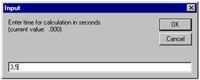
The setting of the steady-state flow takes e.g. 8 seconds. To determine the state of the entire pipe network after e.g. 3,5 seconds select the menu item “Calculate unsteady” – “Give time for calculation”:

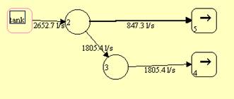
Start the calculation. The result is shown in the mask:

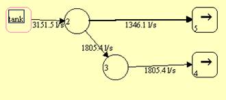
Do you want to determine the course of the flow for a another pressure increase? Select “Repeat pressure change" in the "Calculate unsteady” menu and start the calculation. Consequently, the volume flow is higher now:

The flow curve shows that the final value is reached after approx. five seconds.

The previous calculations started out from the idle state. Supposing you want to start the calculation with a velocity of 2 m/s at the tapping-point fitting or with a corresponding initial volume flow.

Select “Give initial velocity” in the "Calculate unsteady" menu and enter the value 2 (seconds):

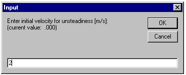
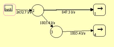
Start the calculation. The final values do not change whereas the steady state is reached earlier: in this example after approx. 4 seconds instead of 5 seconds.

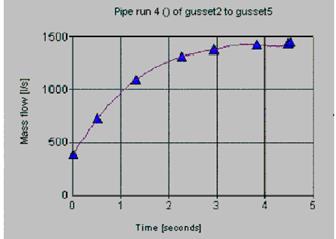
You can determine the time dependent data for another pipe run.

Mark the box “Determine unsteady data for this run” for the pipe run    tank è 3 in the pipe mask and start the calculation.

Note:          This box is displayed only if at least one pipe run has been linked with the module KV before.

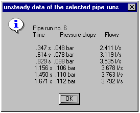
The results are displayed:

in the flow curve and

in the “Calculate unsteady” menu under “Data of the selected runs”:

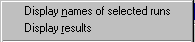
The item "Display results" can be selected as soon as the calculation has been finished. Before that, only the selected run(s) are displayed under "Display names of selected runs".

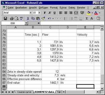
If you have installed WORD 97 (WORD 8.0) or EXCEL 97 (EXCEL 8.0) on your computer you can save the unsteady data directly in DOC or XLS format.

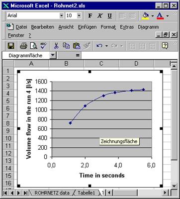
In addition to that, a flow curve is created as diagram in EXCEL automatically.

Using the additional options of the server program enables you to analyse any other correlation.

With the menu item “Calculate unsteady” – “Change into calculation module” you switch to the calculation mask of the server program running in the background.

By modifying the black input values in this mask you can calculate any arrangement. The output values are displayed in blue colour (You can change the display colours if desired).

In the calculation mask of the server program all options like "Print" etc. can be used. Start the ATLAS help in the “Help” menu for further information.

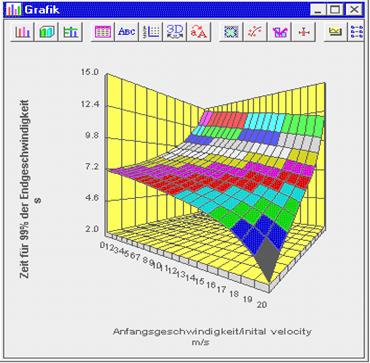
In the “Atlas” menu under “Parameter study” you can analyse the dependencies between two or three values (two- or three-dimensional parameter studies).

With this analysis you can do further examinations going beyond the possibilities of the program ROHRNETZ (PIPE NETWORK).

The following graphics shows – as one of many possible examples – the calculation result for the dependence of the time until reaching 99 % of the end velocity as a function of the loss coefficient of the fitting and the initial velocity (i.e. the initial volume flow). The graphics has been created without any additional help programs, using the calculation module KV only.